


Línguas
Páginas
Legal

Segmentação II
Paulo Sérgio RodriguesPEL205
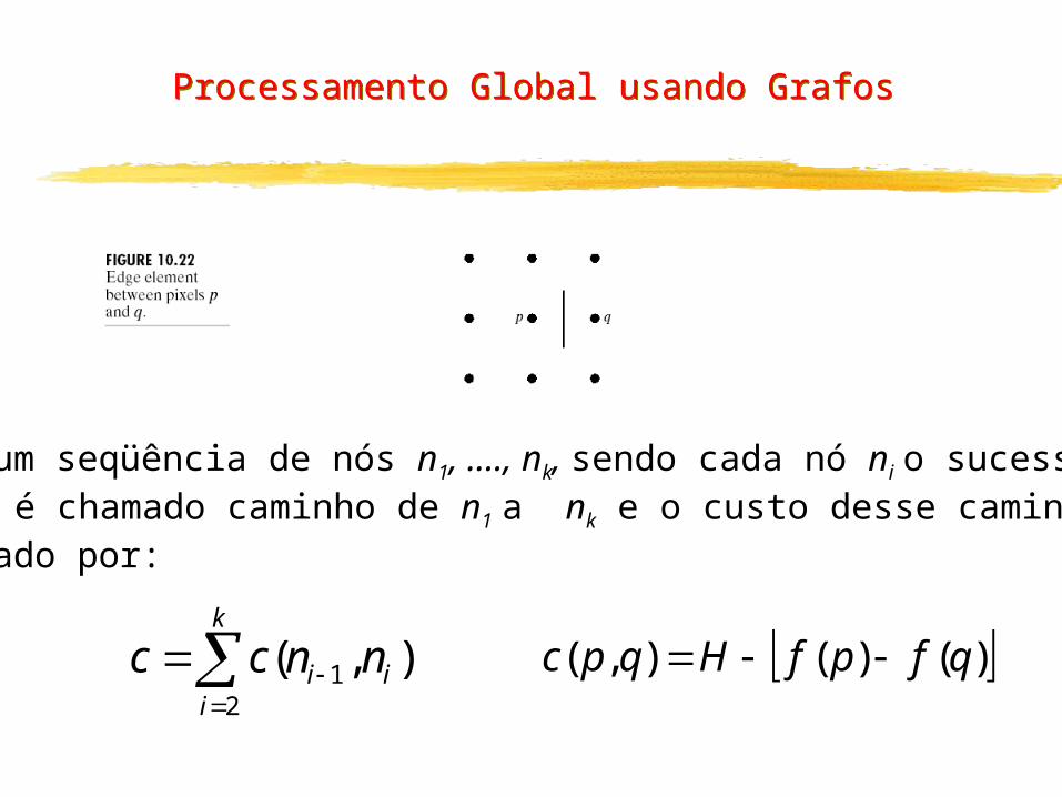
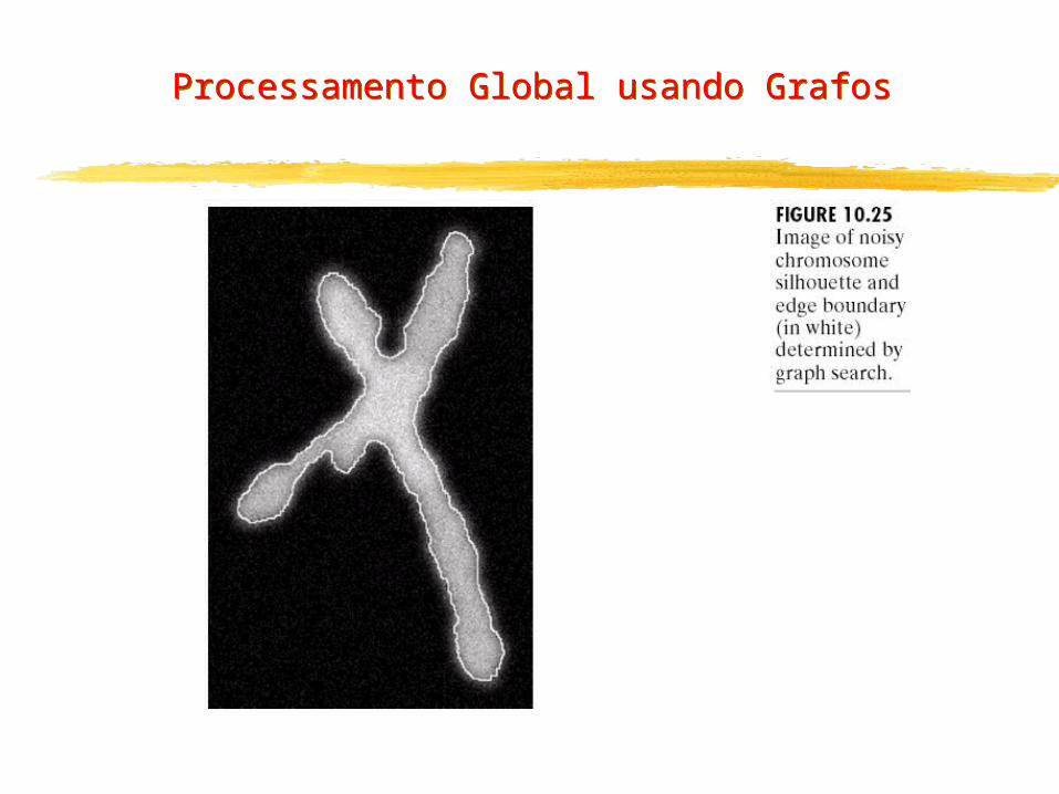
Processamento Global usando Grafos
Para um seqüência de nós n1, ...., nk, sendo cada nó ni o sucessorde ni-1 é chamado caminho de n1 a nk e o custo desse caminho podeser dado por:
k
iii nncc
21 ),( )()(),( qfpfHqpc
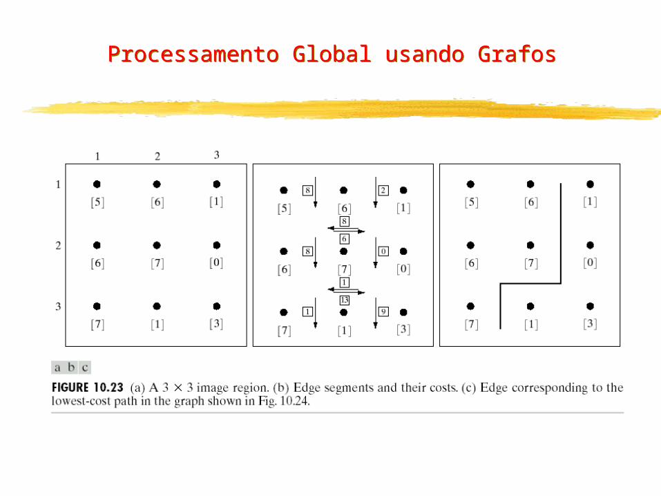
Processamento Global usando Grafos
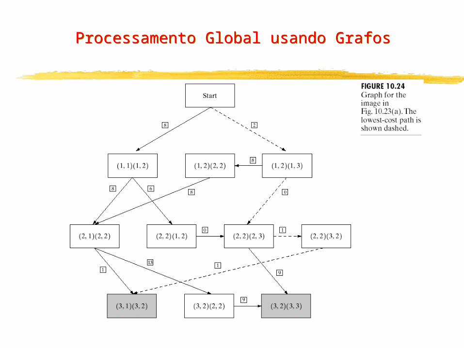
Processamento Global usando Grafos
Processamento Global usando Grafos
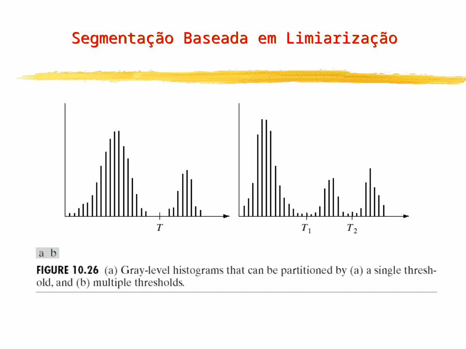
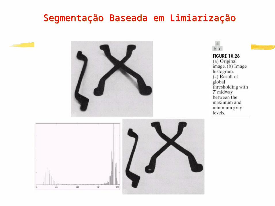
Segmentação Baseada em Limiarização
Segmentação Baseada em Limiarização
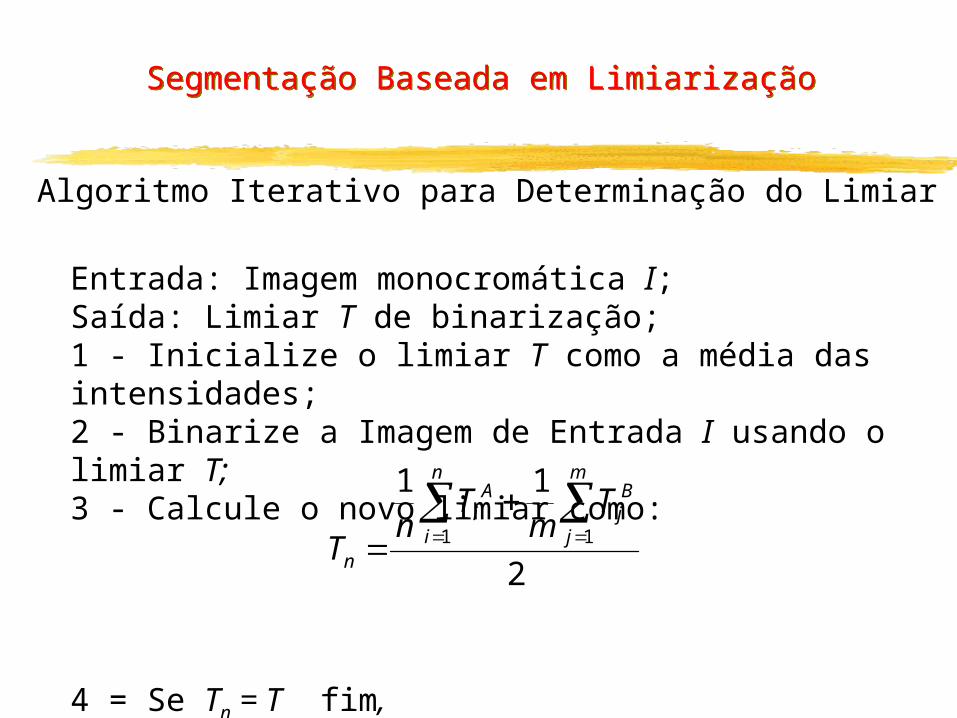
Algoritmo Iterativo para Determinação do Limiar
Entrada: Imagem monocromática I;Saída: Limiar T de binarização;1 - Inicialize o limiar T como a média das intensidades;2 - Binarize a Imagem de Entrada I usando o limiar T;3 - Calcule o novo limiar como:
4 = Se Tn = T fim, caso contrário faça T = Tn e volte ao passo 2;
2
1111
m
j
Bj
n
i
Ai
n
Tm
Tn
T
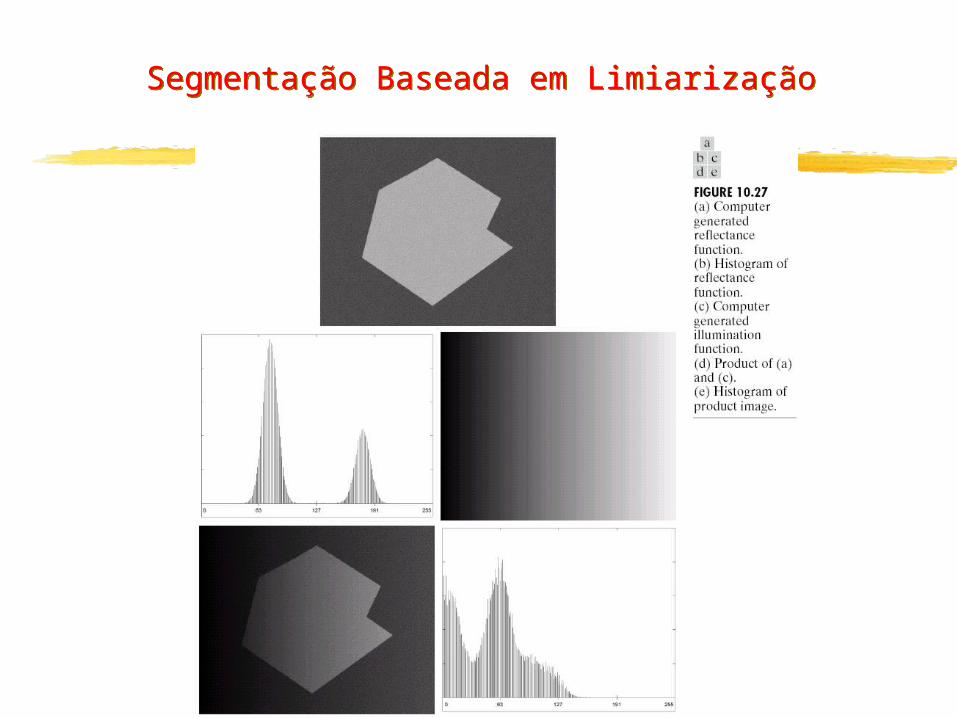
Segmentação Baseada em Limiarização
Segmentação Baseada em Limiarização
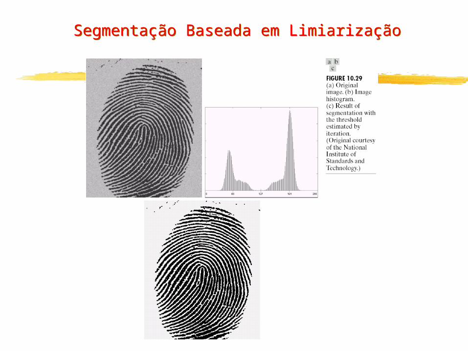
Segmentação Baseada em Limiarização
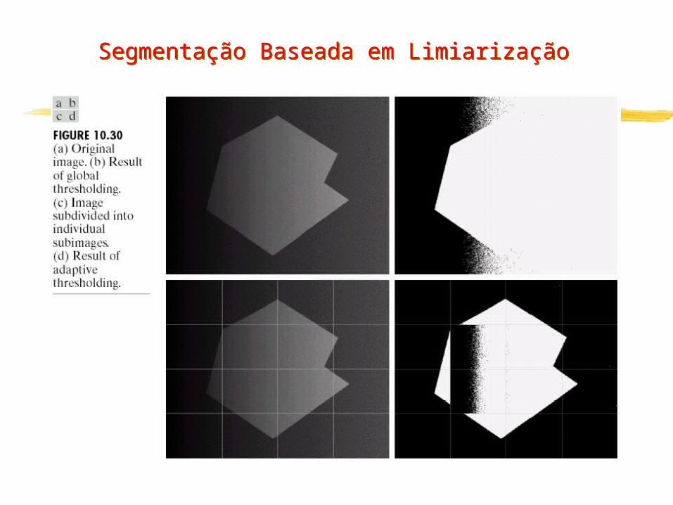
Segmentação Baseada em Limiarização
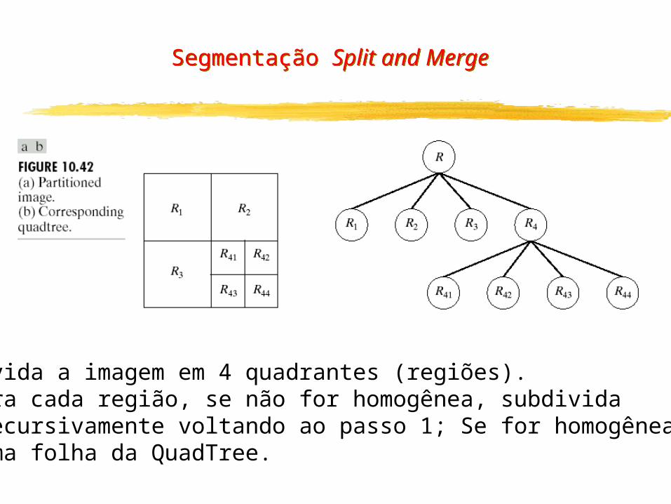
Segmentação Split and Merge
1 - Divida a imagem em 4 quadrantes (regiões).2 - Para cada região, se não for homogênea, subdivida recursivamente voltando ao passo 1; Se for homogênea vira uma folha da QuadTree.
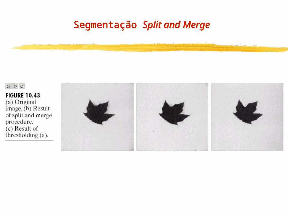
Segmentação Split and Merge
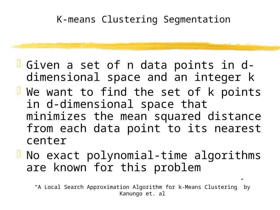
K-means Clustering Segmentation
Given a set of n data points in d-dimensional space and an integer k
We want to find the set of k points in d-dimensional space that minimizes the mean squared distance from each data point to its nearest center
No exact polynomial-time algorithms are known for this problem
“A Local Search Approximation Algorithm for k-Means Clustering” by Kanungo et. al
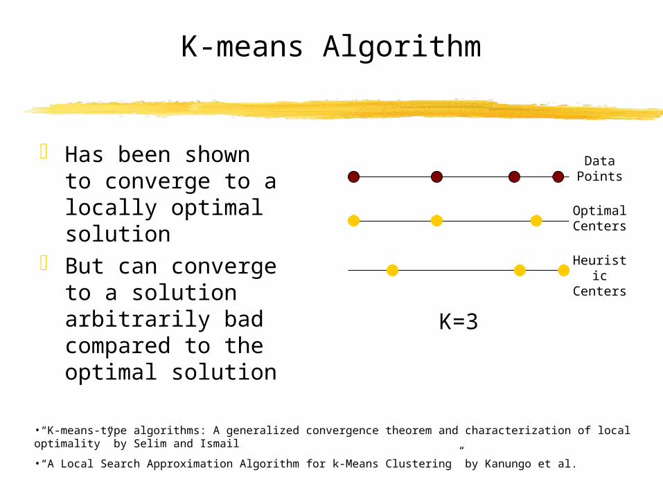
K-means Algorithm
Has been shown to converge to a locally optimal solution
But can converge to a solution arbitrarily bad compared to the optimal solution
•“K-means-type algorithms: A generalized convergence theorem and characterization of local optimality” by Selim and Ismail•“A Local Search Approximation Algorithm for k-Means Clustering” by Kanungo et al.
K=3
Data Points
Optimal Centers
Heuristic Centers
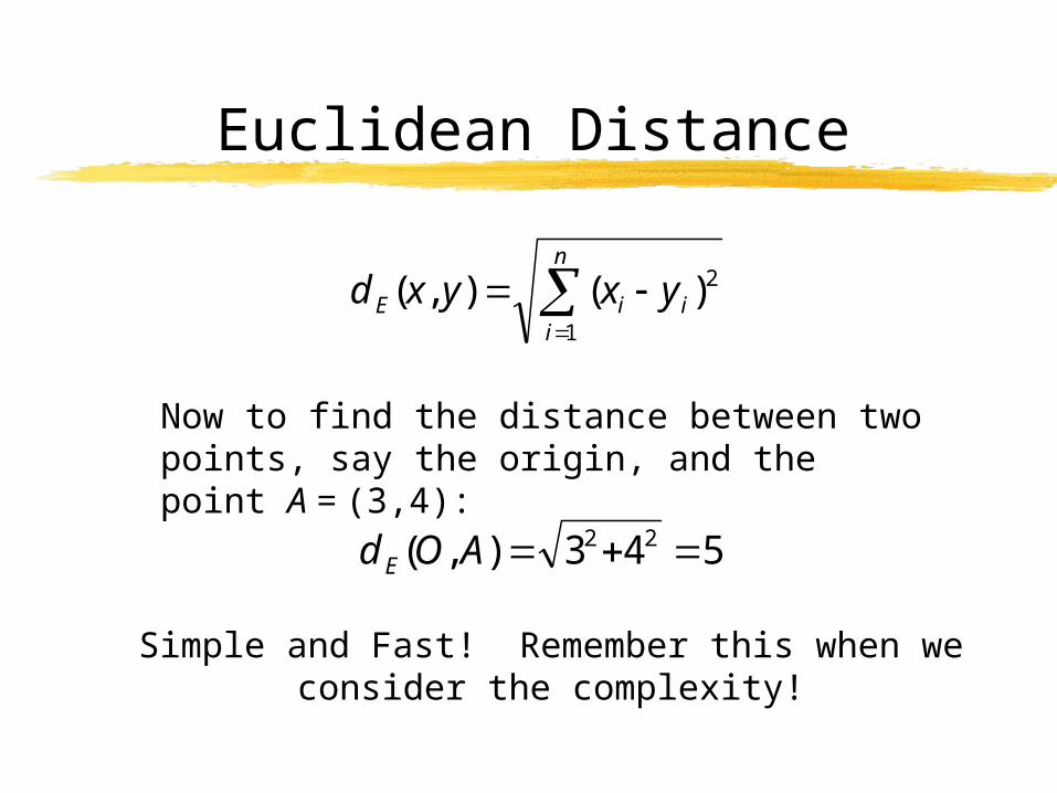
Euclidean Distance
n
iiiE yxyxd
1
2)(),(
543),( 22 AOd E
Now to find the distance between two points, say the origin, and the point A = (3,4):
Simple and Fast! Remember this when we consider the complexity!
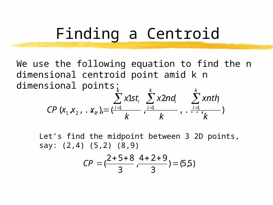
Finding a CentroidWe use the following equation to find the n dimensional centroid point amid k n dimensional points:
),...,2
,1
(),...,,( 11121 k
xnth
k
ndx
k
stxxxxCP
k
ii
k
ii
k
ii
k
Let’s find the midpoint between 3 2D points, say: (2,4) (5,2) (8,9)
)5,5()3
924,3
852(
CP
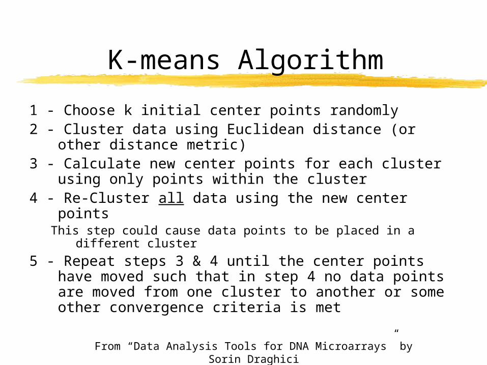
K-means Algorithm1 - Choose k initial center points randomly2 - Cluster data using Euclidean distance (or other
distance metric)3 - Calculate new center points for each cluster using
only points within the cluster4 - Re-Cluster all data using the new center points
This step could cause data points to be placed in a different cluster
5 - Repeat steps 3 & 4 until the center points have moved such that in step 4 no data points are moved from one cluster to another or some other convergence criteria is met
From “Data Analysis Tools for DNA Microarrays” by Sorin Draghici
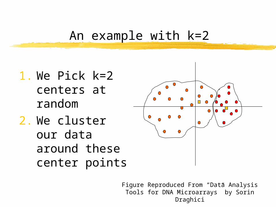
An example with k=2
1. We Pick k=2 centers at random
2. We cluster our data around these center points
Figure Reproduced From “Data Analysis Tools for DNA Microarrays” by Sorin Draghici
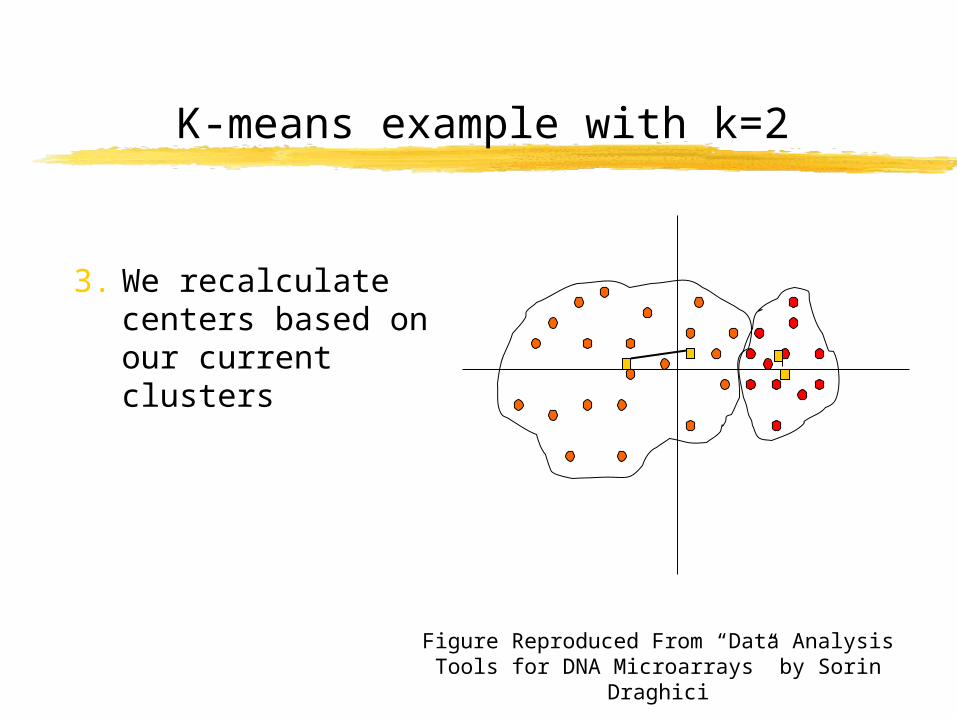
K-means example with k=2
3. We recalculate centers based on our current clusters
Figure Reproduced From “Data Analysis Tools for DNA Microarrays” by Sorin Draghici
K-means example with k=2
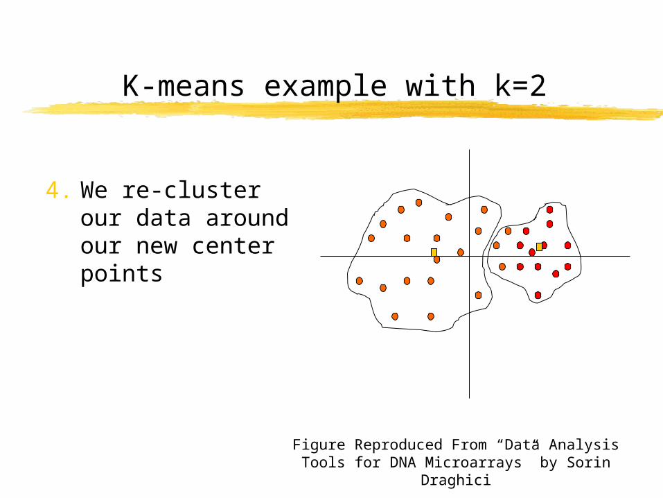
4. We re-cluster our data around our new center points
Figure Reproduced From “Data Analysis Tools for DNA Microarrays” by Sorin Draghici
K-means example with k=2
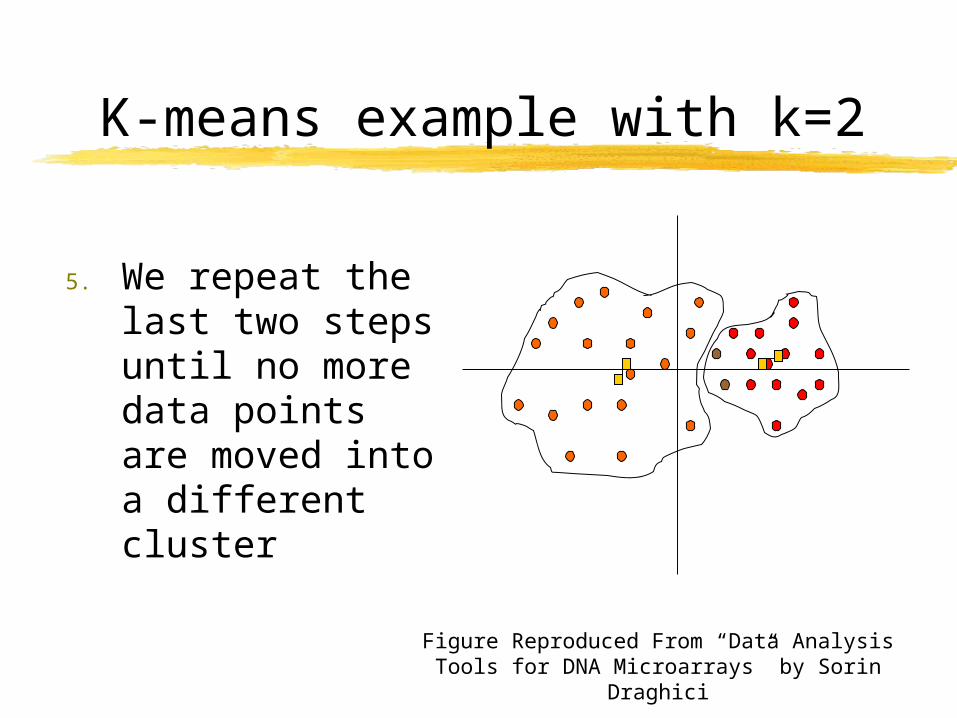
5. We repeat the last two steps until no more data points are moved into a different cluster
Figure Reproduced From “Data Analysis Tools for DNA Microarrays” by Sorin Draghici
Characteristics of k-means Clustering
The random selection of initial center points creates the following properties Non-Determinism May produce clusters without patterns
One solution is to choose the centers randomly from existing patterns
From “Data Analysis Tools for DNA Microarrays” by Sorin Draghici
Algorithm ComplexityLinear in the number of data points,
NCan be shown to have time of cN
c does not depend on N, but rather the number of clusters, k
Low computational complexityHigh speed
From “Data Analysis Tools for DNA Microarrays” by Sorin Draghici
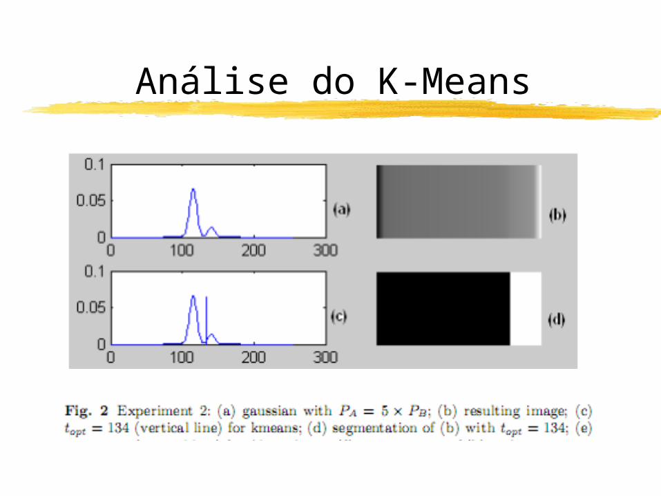
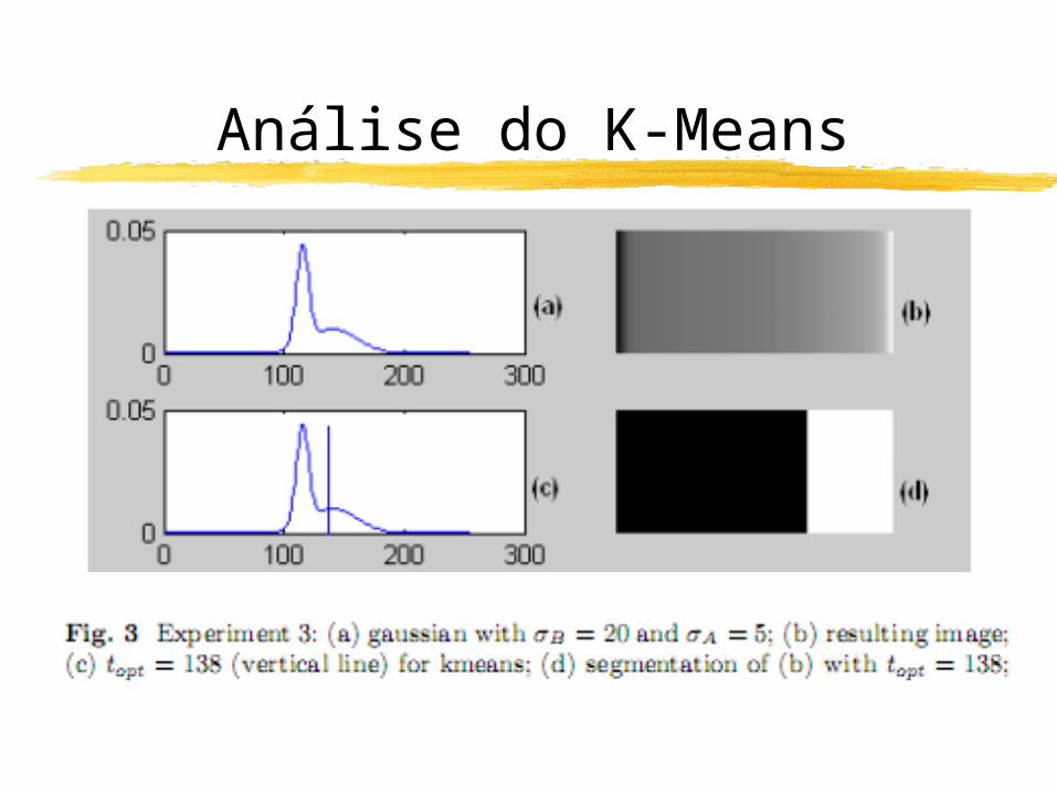
Análise do K-Means
Análise do K-Means
• Entropia Tradicional BGS
• q-Entropia
• Aplicações da q-entropia à PDI
Segmentação Baseada em Entropia
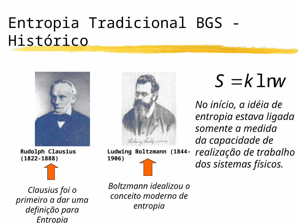
Entropia Tradicional BGS - Histórico
Rudolph Clausius (1822-1888)
Clausius foi o primeiro a dar uma definição
para Entropia
Ludwing Boltzmann (1844-1906)
Boltzmann idealizou o conceito moderno de
entropia
wkS lnNo início, a idéia deentropia estava ligadasomente a medidada capacidade de realização de trabalhodos sistemas físicos.
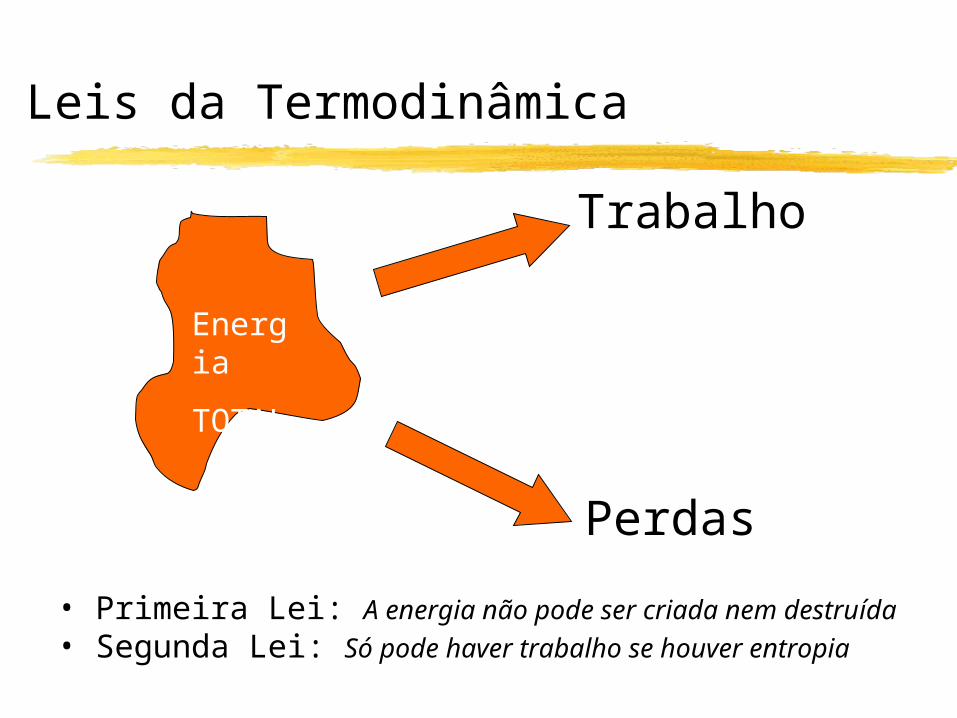
Leis da Termodinâmica
Trabalho
Perdas
Energia
TOTAL
• Primeira Lei: A energia não pode ser criada nem destruída • Segunda Lei: Só pode haver trabalho se houver entropia
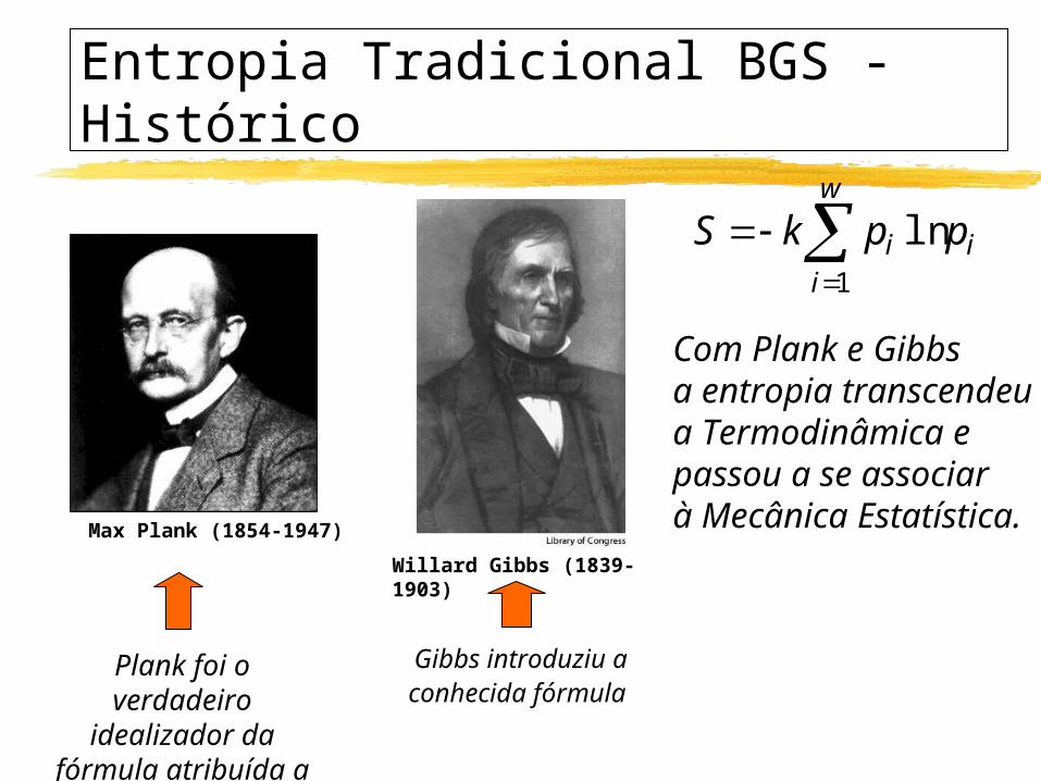
Max Plank (1854-1947)
Plank foi o verdadeiro idealizador da fórmula atribuída a Boltzmann
Willard Gibbs (1839-1903)
Gibbs introduziu a conhecida fórmula
w
iii ppkS
1
ln
Com Plank e Gibbsa entropia transcendeua Termodinâmica epassou a se associar à Mecânica Estatística.
Entropia Tradicional BGS - Histórico
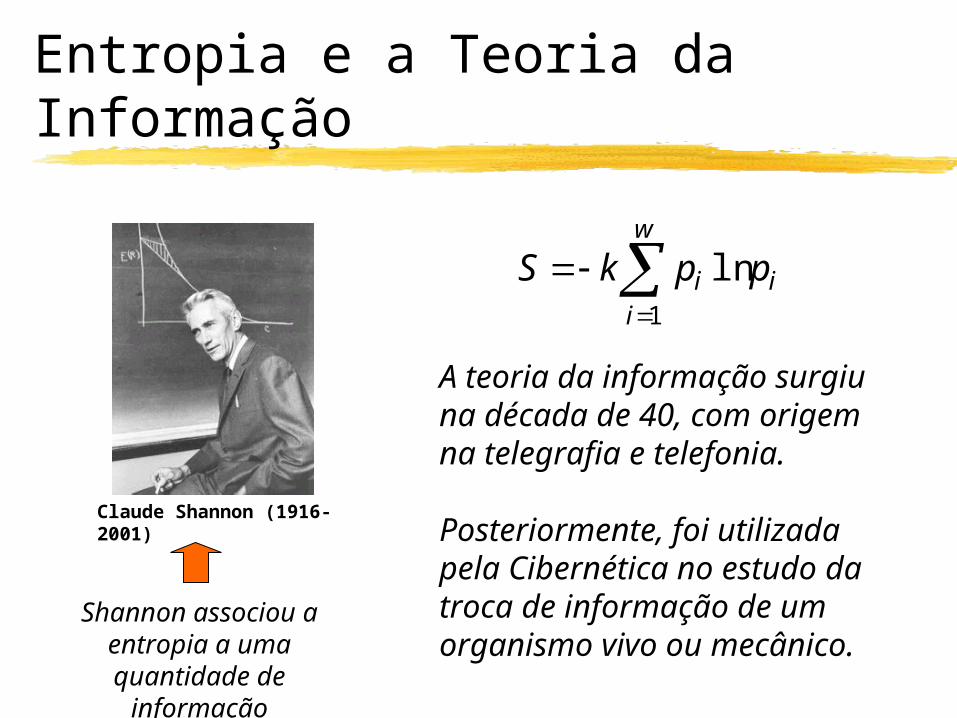
Entropia e a Teoria da Informação
Claude Shannon (1916-2001)
Shannon associou a entropia a uma
quantidade de informação
A teoria da informação surgiuna década de 40, com origemna telegrafia e telefonia.
Posteriormente, foi utilizada pela Cibernética no estudo datroca de informação de um organismo vivo ou mecânico.
w
iii ppkS
1
ln
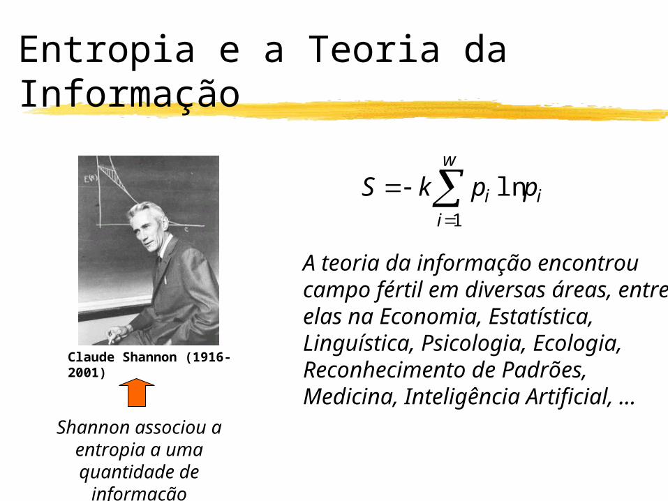
Entropia e a Teoria da Informação
Claude Shannon (1916-2001)
Shannon associou a entropia a uma
quantidade de informação
A teoria da informação encontrou campo fértil em diversas áreas, entreelas na Economia, Estatística, Linguística, Psicologia, Ecologia,Reconhecimento de Padrões, Medicina, Inteligência Artificial, ...
w
iii ppkS
1
ln
Generalização da Entropia Clássica
• Sabe-se há mais de um século que entropia tradicional de BG não é capaz de explicar determinados Sistemas Físicos
• Tais sistemas possuem como características:- interações espaciais de longo alcance- interações temporais de longo alcance- comportamento fractal nas fronteiras
• E são chamados de Sistemas Não-Extensivos
Generalização da Entropia Clássica
• Exemplos
• turbulência• massa e energia das galáxias• Lei de Zipf-Mandelbrot da linguística• Teoria de risco financeiro
Generalização da Entropia Clássica
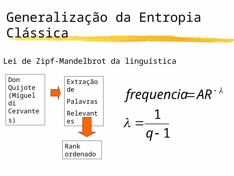
• Lei de Zipf-Mandelbrot da linguística
11
q
ARfrequencia
Don Quijote (Miguel di Cervantes)
Extração de
Palavras
Relevantes
Rank ordenado
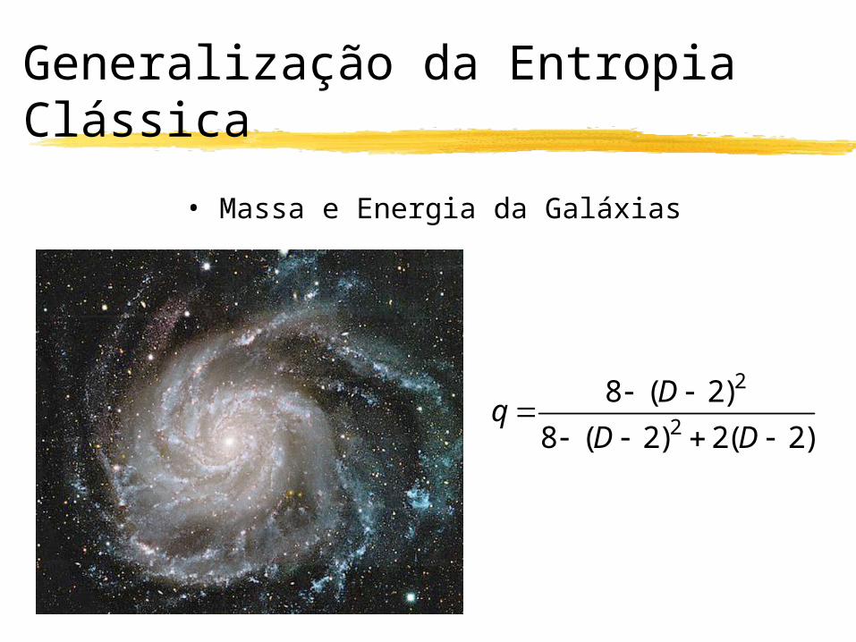
Generalização da Entropia Clássica
• Massa e Energia da Galáxias
)2(2)2(8)2(8
2
2
DD
Dq
Generalização da Entropia Clássica
• Teoria do Risco Financeiro
• Quando se tem expectativa de perda, algumas pessoas preferem arriscar
• Quando se tem expectativa de ganho, algumas pessoas preferem não arriscar
Generalização da Entropia Clássica
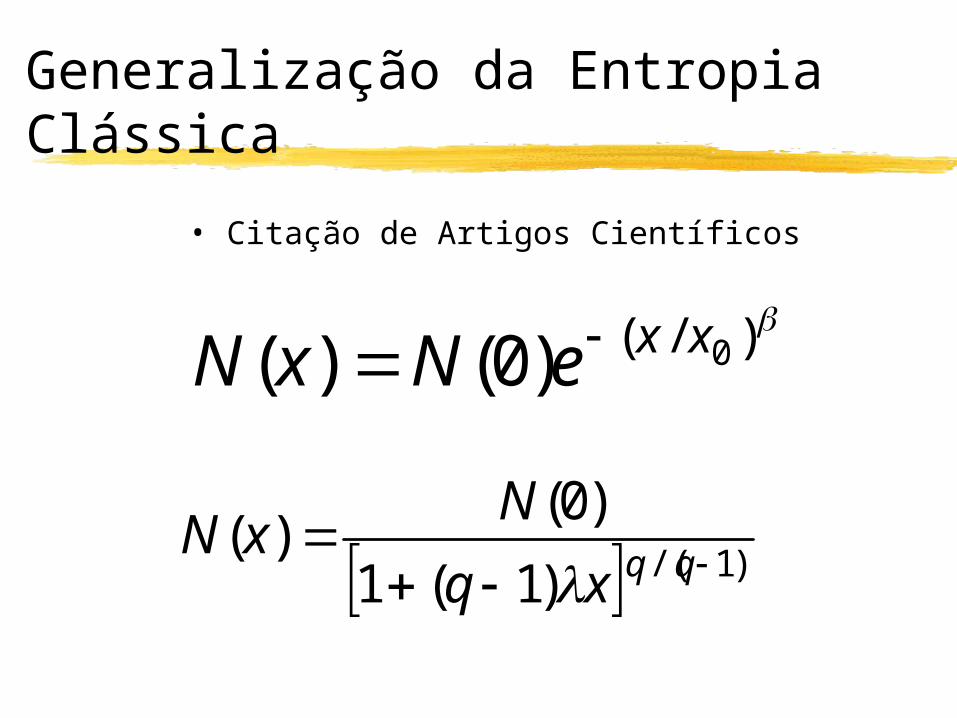
• Citação de Artigos Científicos
)/( 0)0()( xxeNxN
)1/()1(1)0()(
qqxq
NxN
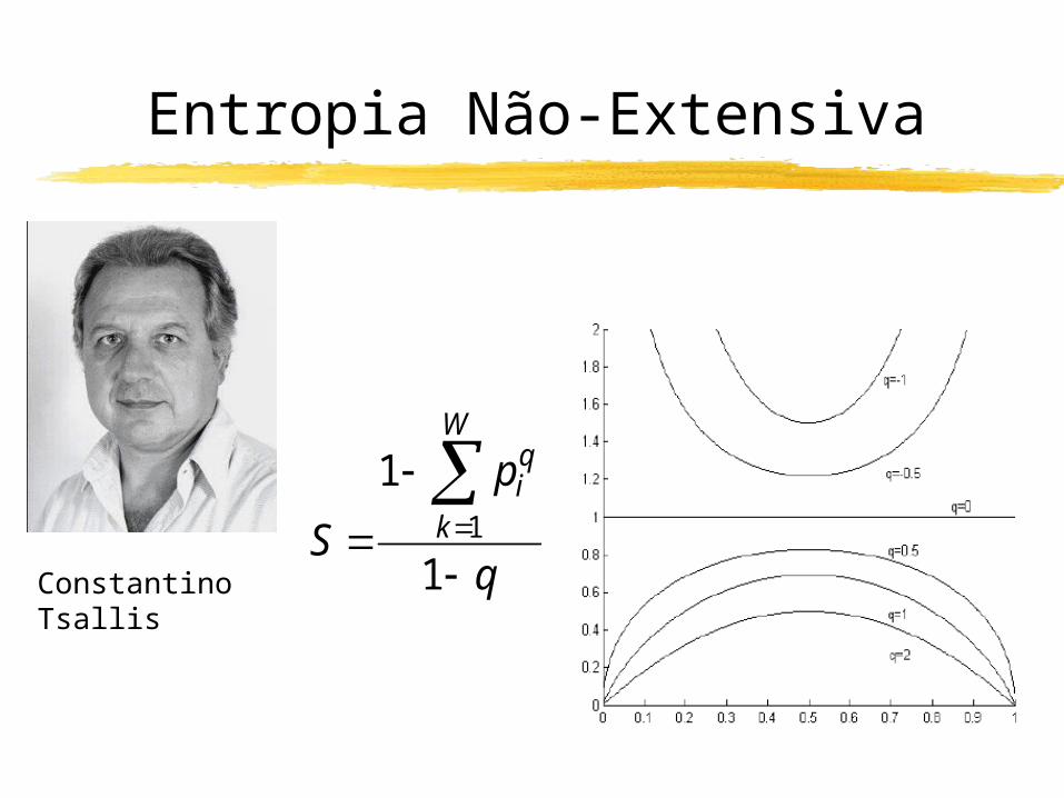
Entropia Não-Extensiva
q
p
S
W
k
qi
1
11
Constantino Tsallis
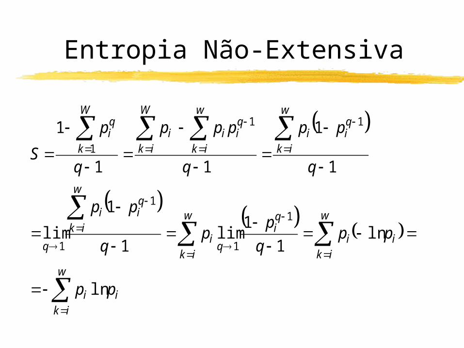
Entropia Não-Extensiva
w
ikii
w
ikii
qi
q
w
iki
w
ik
qii
q
w
ik
qii
w
ik
qii
W
iki
W
k
qi
pp
ppq
pp
q
pp
q
pp
q
ppp
q
p
S
ln
ln1
1lim
1
1
lim
1
1
11
1
1
1
1
1
11
1
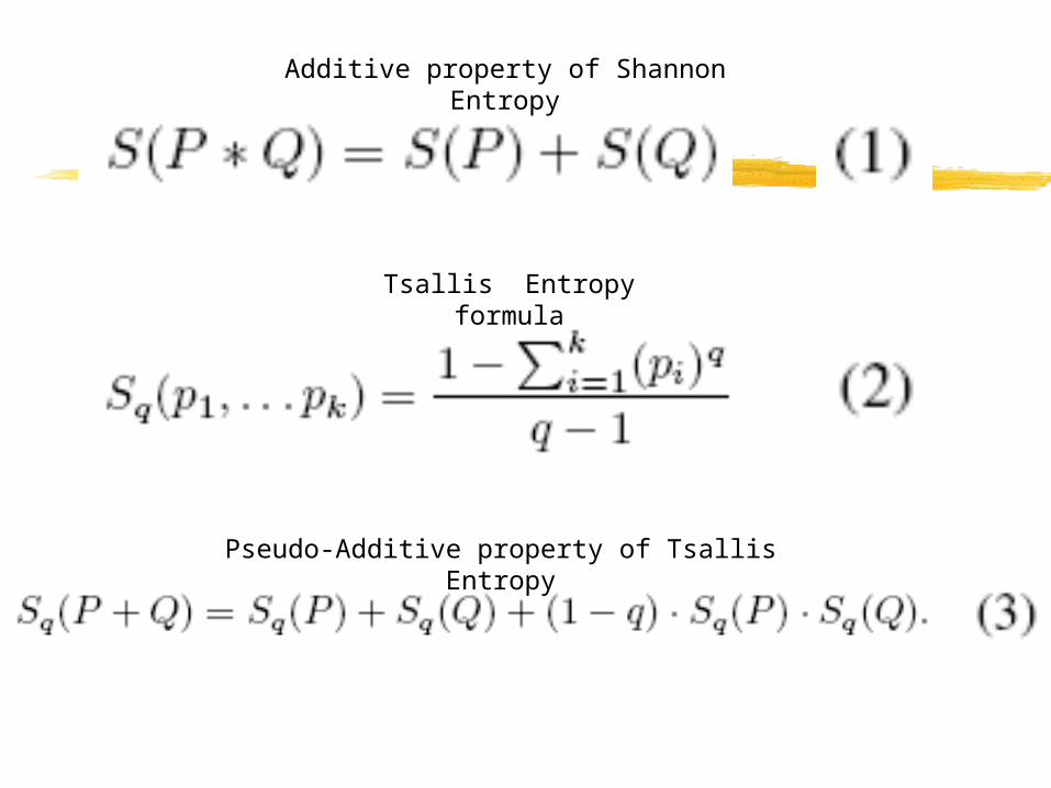
Additive property of Shannon Entropy
Tsallis Entropy formula
Pseudo-Additive property of Tsallis Entropy
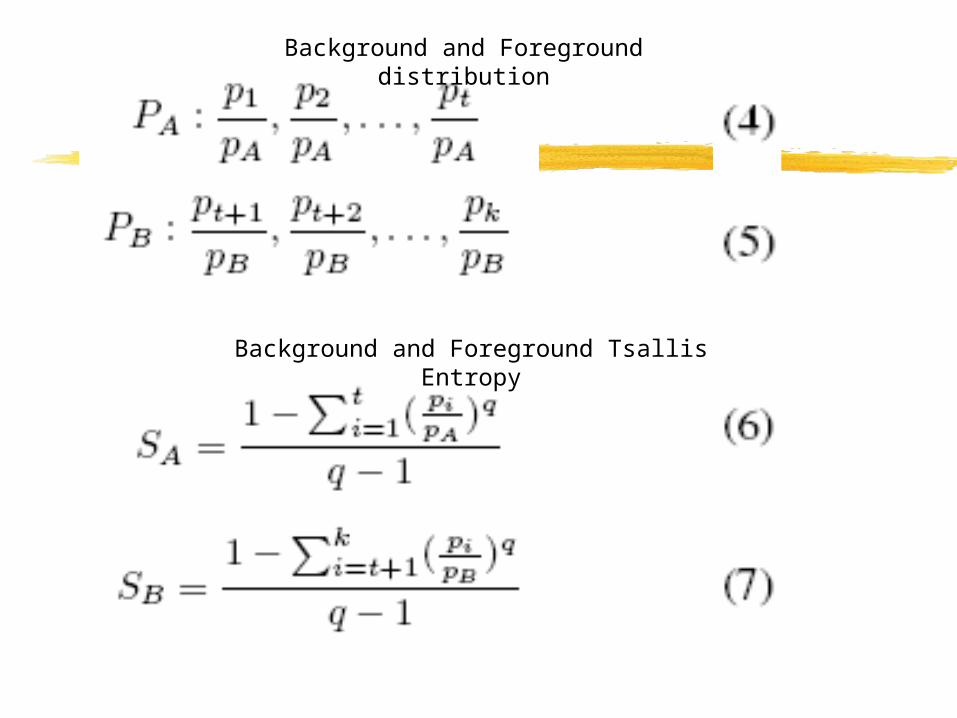
Background and Foreground distribution
Background and Foreground Tsallis Entropy
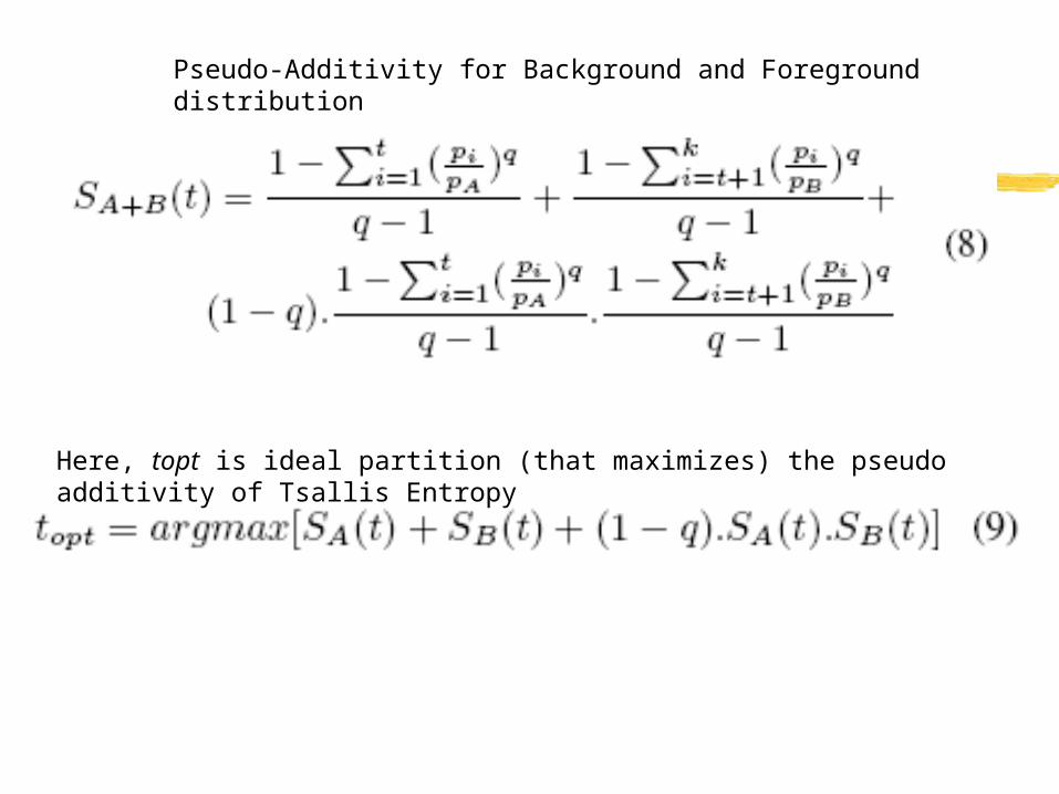
Pseudo-Additivity for Background and Foreground distribution
Here, topt is ideal partition (that maximizes) the pseudo additivity of Tsallis Entropy
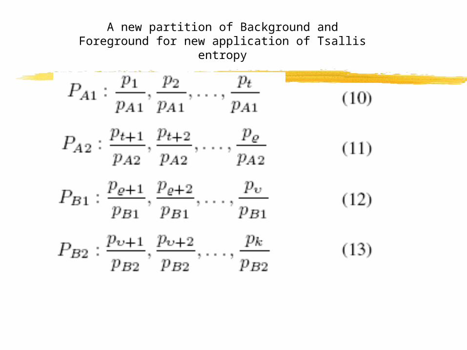
A new partition of Background and Foreground for new application of Tsallis entropy
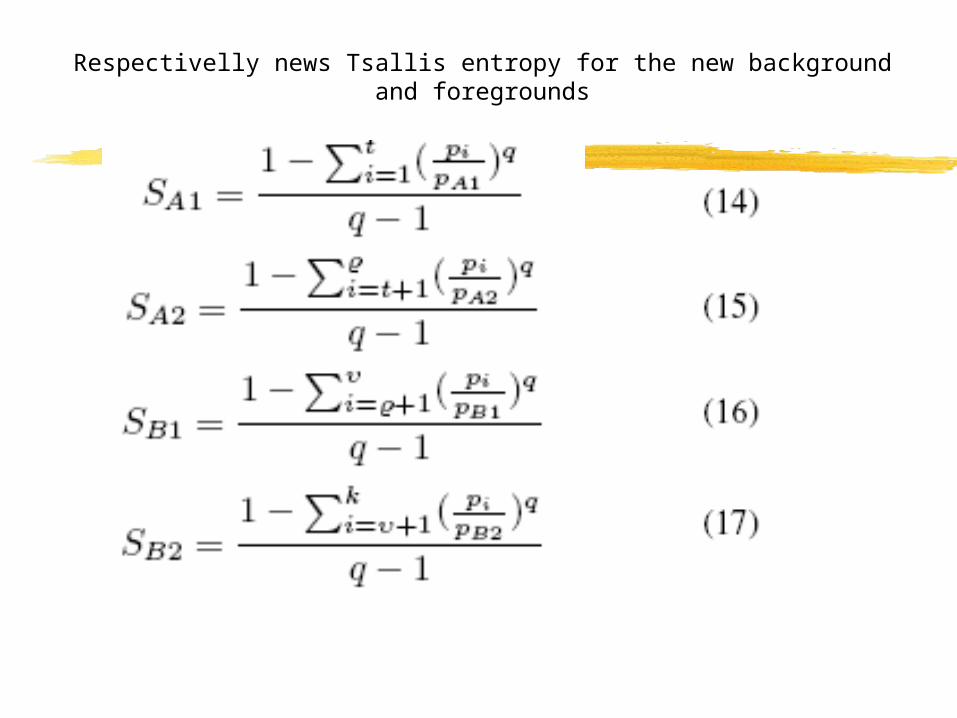
Respectivelly news Tsallis entropy for the new background and foregrounds
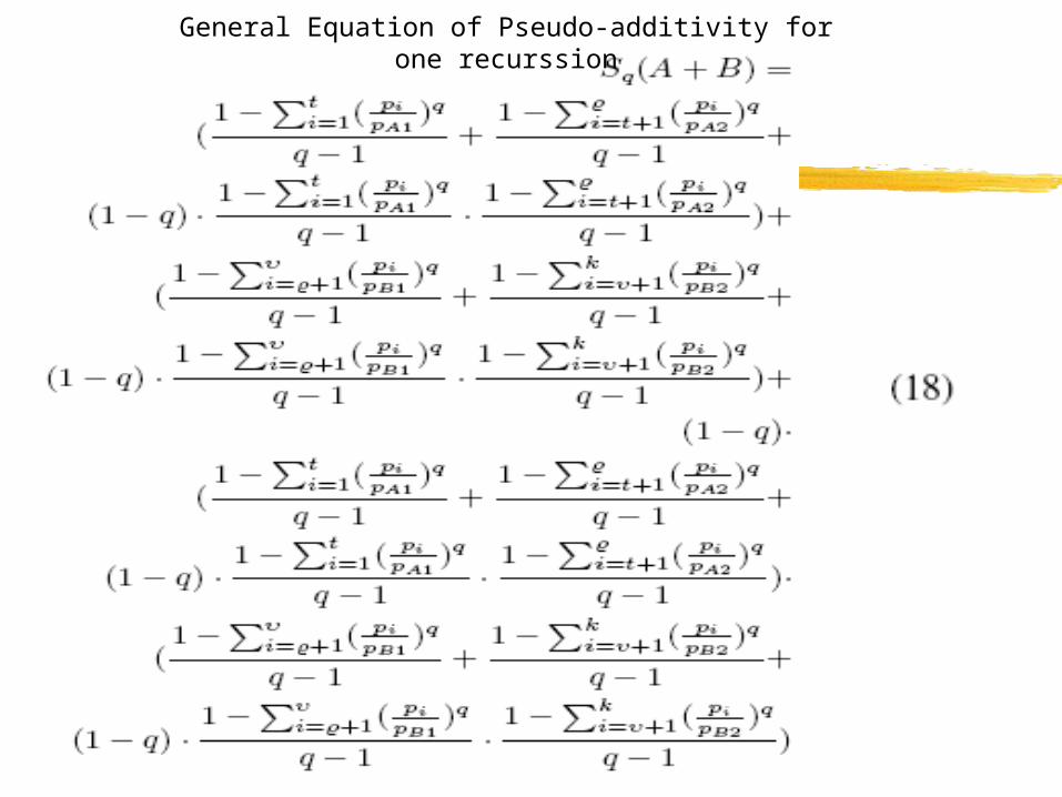
General Equation of Pseudo-additivity for one recurssion
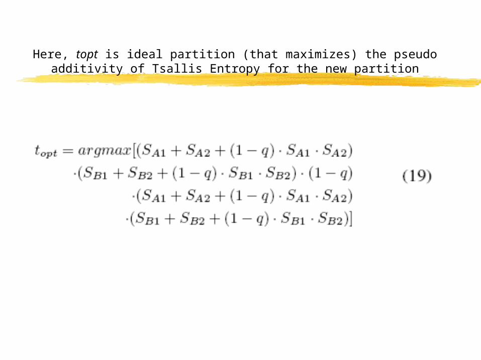
Here, topt is ideal partition (that maximizes) the pseudo additivity of Tsallis Entropy for the new partition
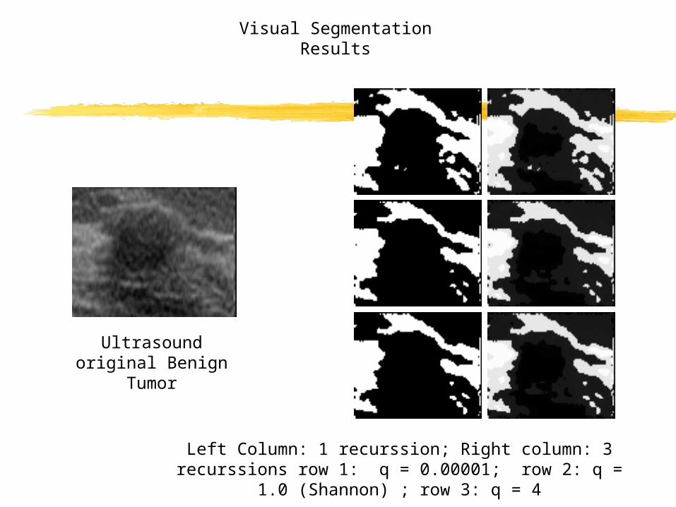
Ultrasound original Benign Tumor
Left Column: 1 recurssion; Right column: 3 recurssions row 1: q = 0.00001; row 2: q = 1.0 (Shannon) ; row 3: q = 4
Visual Segmentation Results
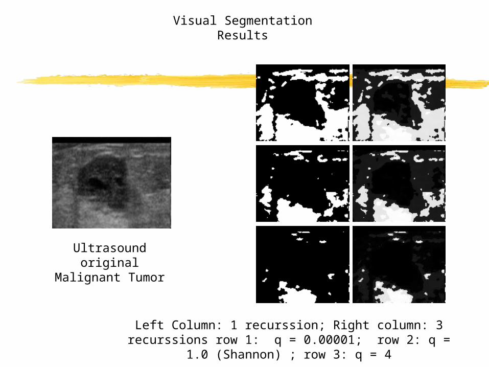
Left Column: 1 recurssion; Right column: 3 recurssions row 1: q = 0.00001; row 2: q = 1.0 (Shannon) ; row 3: q = 4
Ultrasound original Malignant Tumor
Visual Segmentation Results
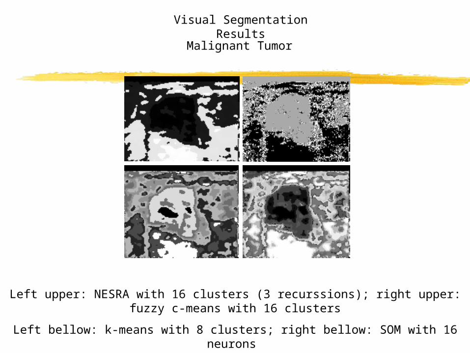
Left upper: NESRA with 16 clusters (3 recurssions); right upper: fuzzy c-means with 16 clusters
Left bellow: k-means with 8 clusters; right bellow: SOM with 16 neurons
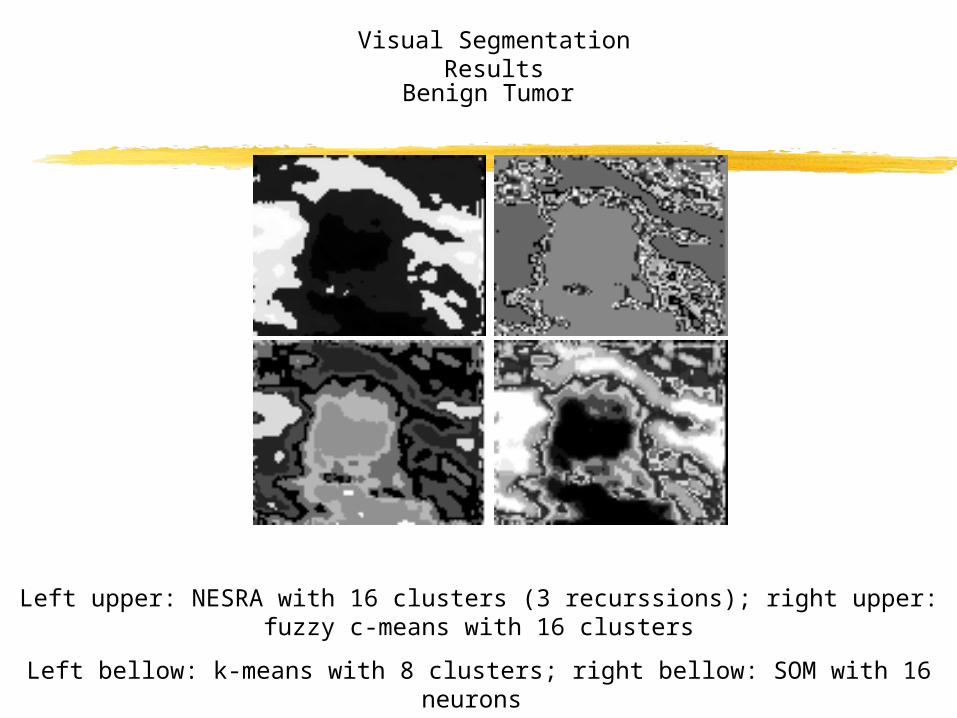
Visual Segmentation Results
Benign Tumor
Left upper: NESRA with 16 clusters (3 recurssions); right upper: fuzzy c-means with 16 clusters
Left bellow: k-means with 8 clusters; right bellow: SOM with 16 neurons
Visual Segmentation Results
Malignant Tumor
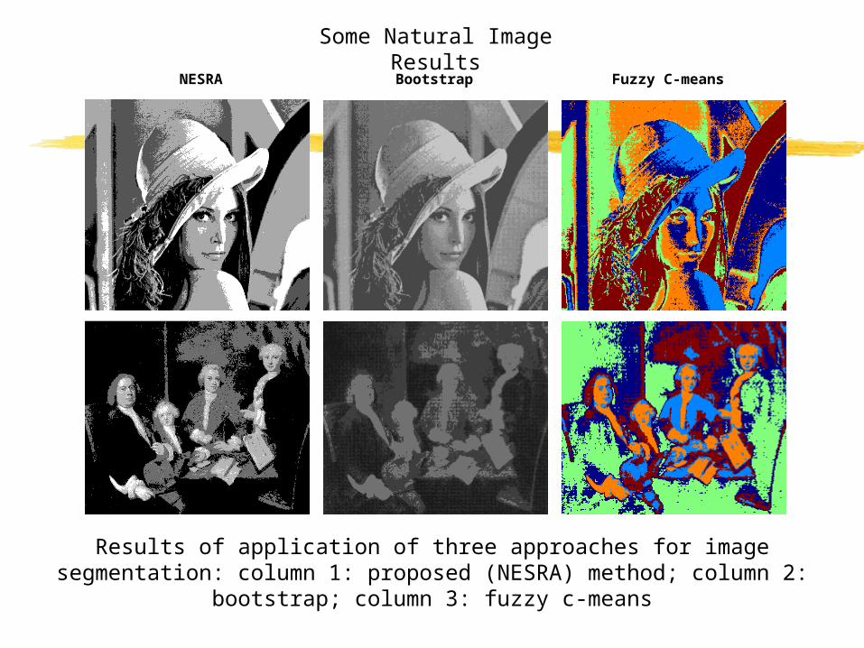
Results of application of three approaches for imagesegmentation: column 1: proposed (NESRA) method; column 2: bootstrap; column 3:
fuzzy c-means
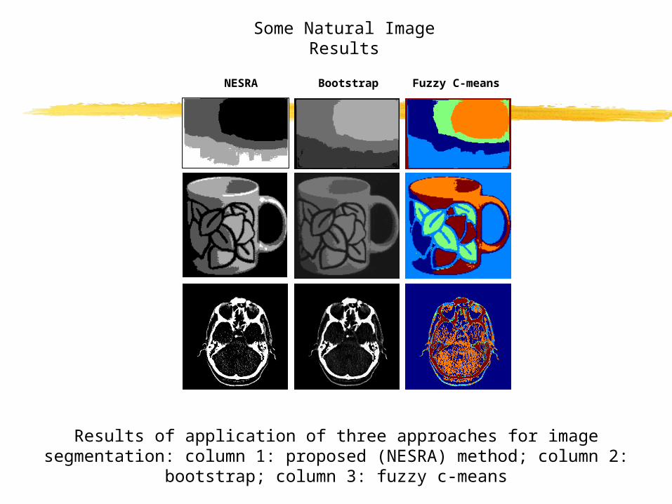
Some Natural Image Results
NESRA Bootstrap Fuzzy C-means
Results of application of three approaches for imagesegmentation: column 1: proposed (NESRA) method; column 2: bootstrap; column 3:
fuzzy c-means
Some Natural Image Results
NESRA Bootstrap Fuzzy C-means
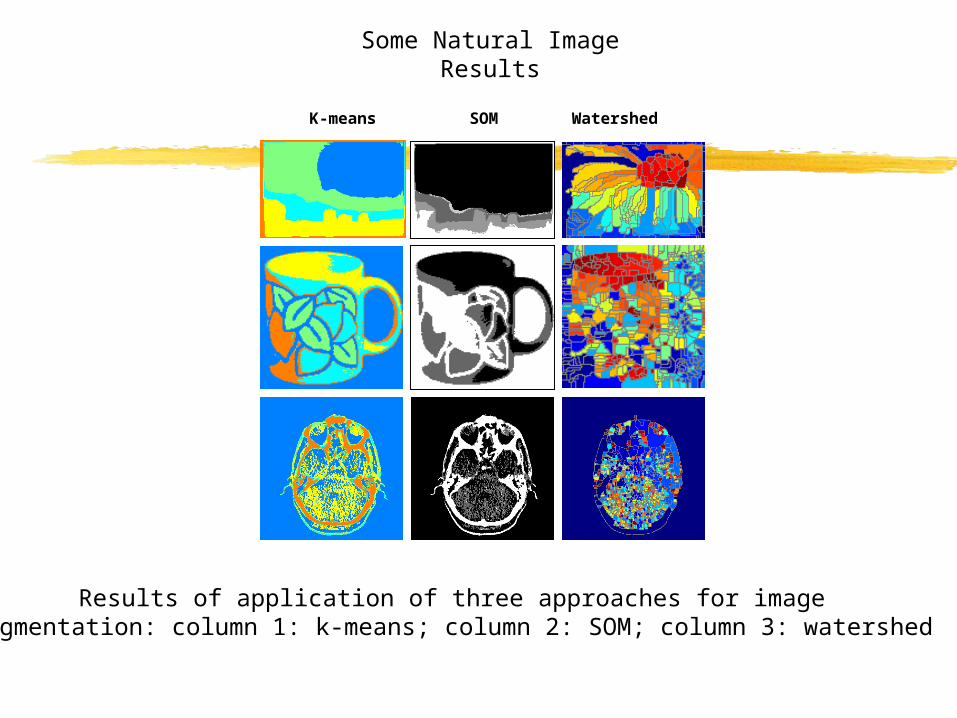
Results of application of three approaches for imagesegmentation: column 1: k-means; column 2: SOM; column 3: watershed
Some Natural Image Results
K-means SOM Watershed
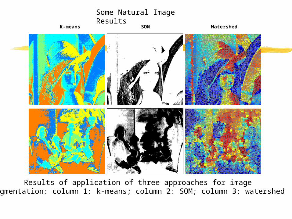
Results of application of three approaches for imagesegmentation: column 1: k-means; column 2: SOM; column 3: watershed
Some Natural Image Results
K-means SOM Watershed
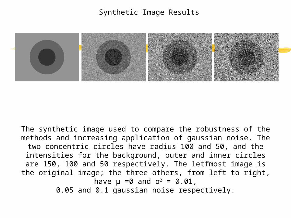
The synthetic image used to compare the robustness of the methods and increasing application of gaussian noise. The two concentric circles have radius 100 and 50, and the intensities for the background, outer and inner circles are
150, 100 and 50 respectively. The letfmost image is the original image; the three others, from left to right, have μ =0 and σ2 = 0.01,
0.05 and 0.1 gaussian noise respectively.
Synthetic Image Results
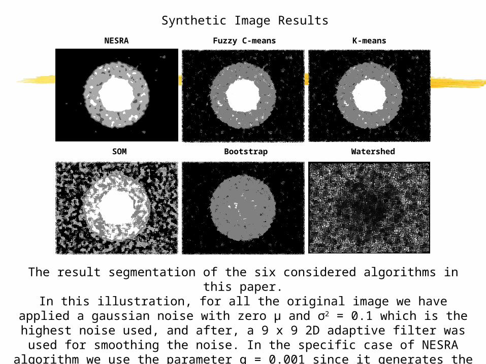
The result segmentation of the six considered algorithms in this paper.In this illustration, for all the original image we have applied a gaussian noise with zero μ and σ2 = 0.1 which is the highest noise used, and after, a 9 x 9 2D adaptive filter was
used for smoothing the noise. In the specific case of NESRA algorithm we use the parameter q = 0.001 since it generates the best visual result with more homogeneous
and noiseless regions.
Synthetic Image ResultsNESRA
Bootstrap
Fuzzy C-means K-means
SOM Watershed
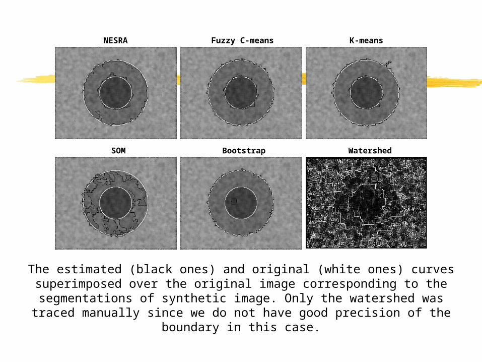
The estimated (black ones) and original (white ones) curves superimposed over the original image corresponding to the segmentations of synthetic image. Only the watershed was traced manually since we do not have good precision of the
boundary in this case.
NESRA
Bootstrap
Fuzzy C-means K-means
SOM Watershed
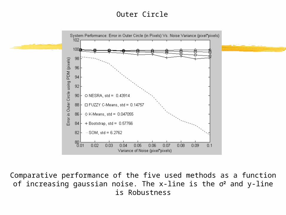
Comparative performance of the five used methods as a function of increasing gaussian noise. The x-line is the σ2 and y-line is Robustness
Outer Circle
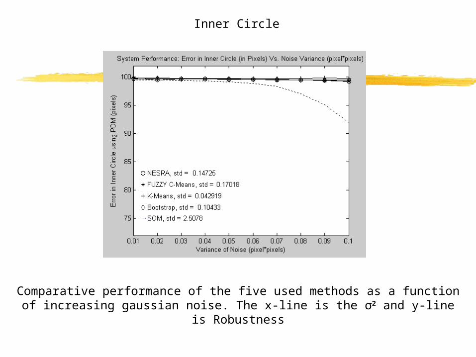
Comparative performance of the five used methods as a function of increasing gaussian noise. The x-line is the σ2 and y-line is Robustness
Inner Circle
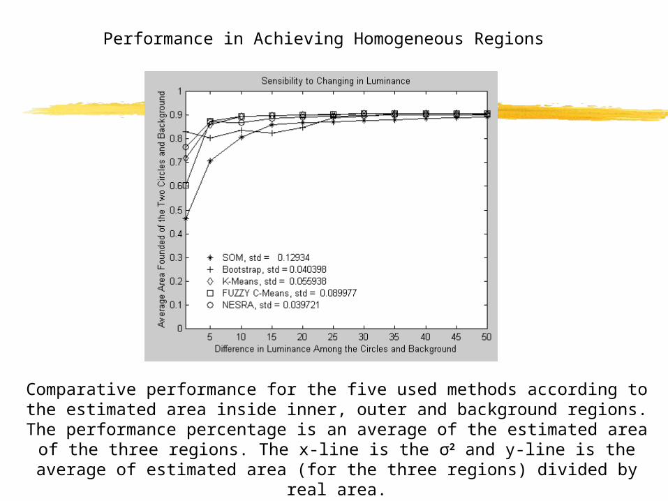
Comparative performance for the five used methods according to the estimated area inside inner, outer and background regions. The performance percentage is an
average of the estimated area of the three regions. The x-line is the σ2 and y-line is the average of estimated area (for the three regions) divided by real area.
Performance in Achieving Homogeneous Regions
Top Related