Aplicação de inversão magnética 3D em baixas latitudes ...
83
Aplicação de inversão magnética 3D em baixas latitudes magnéticas em corpos com remanência – O estudo de caso das formações ferríferas bandadas do Depósito do Pelado, Greenstone Belt Vila Nova , Amapá Dissertação de mestrado em Geologia nº 324 João Paulo Gomes de Souza Orientadora: Prof. Dra. Adalene Moreira Silva Co-orientadora: Prof. Dra. Catarina Labouré Bemfica Toledo Brasília – DF Julho de 2014
Transcript of Aplicação de inversão magnética 3D em baixas latitudes ...

Aplicação de inversão magnética 3D em baixas latitudes magnéticas em corpos com remanência – O estudo de caso das formações ferríferas bandadas do Depósito do Pelado, Greenstone Belt Vila Nova , Amapá
Dissertação de mestrado em Geologia nº 324
João Paulo Gomes de Souza
Orientadora: Prof. Dra. Adalene Moreira Silva
Co-orientadora: Prof. Dra. Catarina Labouré Bemfica Toledo
Brasília – DF
Julho de 2014
2
João Paulo Gomes de Souza
Aplicação de inversão magnética 3D em baixas latitudes magnéticas em corpos com forte remanência – O estudo de caso das formações ferríferas bandadas do Depósito do Pelado, Greenstone Belt Vila Nova , Amapá
Dissertação apresentada ao Programa de Pós-Graduação em Geologia do Instituto de Geociências da Universidade de Brasília
Área de concentração: Prospecção e Geologia Econômica
Orientadora:
Prof. Dra. Adalene Moreira Silva (Unb)
Co-orientadora:
Prof. Dra. Catarina Labouré B. Toledo (UnB)
Banca examinadora
Prof. Dra. Adalene Moreira Silva (UnB)
Prof. Dr. Carlos Alberto Mendonça (IAG/USP)
Prof. Dr. Weligton Rodrigues Borges (Unb)
Brasília – DF
Julho de 2014

3
“Por que cometer erros antigos se há tanto novos há escolher?”
Bertrand Russel

4
AGRADECIMENTOS
A Prof.ª Dra. Adalene Silva pela orientação, motivação e valiosas discussões ao logo desse
trabalho. A Prof.ª Dra. Catarlina Toledo pela dedicação e paciência durante as revisões e discussões do
artigo.
Aos geólogos Pérsio Mandetta e Carlos Alexandre Sousa pelas discussões e apoio, a CPRM por
disponibilizar aos dados aerogeofísicos utilizados nessa tese. Ao geólogo Flavio Freitas pelo material de
geologia disponibilizado para a pesquisa.
Ao geofísico Canditiano Freitas pelo entusiasmo pela geofísica de exploração e pela motivação.
Ao Instituto de Geociências da Universidade de Brasília pela oportunidade de realização deste
trabalho.
A empresa Vale S/A pela liberação dos códigos MAG3D e AMP3D, sem os quais esse trabalho
não poderia ter sido realizado.
A minha família pela compreensão e incentivo, principalmente ao meu pai, do qual herdei o
amor aos estudos.
Aos meus amigos Willan da Silva e Daniel Brake pela ajuda na revisão do texto.
A minha esposa Ingrid Guimaraes pelo apoio, paciência e compreensão ao logo de todo esse
trabalho.

5
RESUMO
As formações ferríferas do Depósito do Pelado estão inseridas na sequência vulcânica-sedimentar do
Grupo Vila Nova no domínio geológico conhecido como Terreno Antigo Cupixi-Tartarugal Grande, no
estado do Amapá. A imagem de intensidade magnética mostra uma anomalia com forte magnetização
remanescente localizado em baixa latitude magnética, o que dificulta a aplicação da redução ao polo e
consequentemente uma inversão por propriedade física, devido a direção da magnetização total não ser
conhecida. Optou-se por aplicar transformações de campo com fraca dependência da direção de
magnetização como amplitude do campo magnético anômalo (AMCA), sinal analítico da integral vertical
(ASVI) e a integral vertical de sinal analítico (VIAS) com o objetivo de obter a correta distribuição da
susceptibilidade para a formação ferrífera em sub-superfície atraves da inversão magnética. Foi-se
utilizado o software MAG3D e AMP3D para a realização de três inversões sintéticas e três inversões
(com dados reais),com as transformações de campo mencionadas anteriormente. Os resultados dos dados
reais foram comparados com os dados de furos da sondagem exploratória e os dados de susceptibilidade
magnética obtidos por perfilagem dos testemunhos de sondagem. Os resultados mostram que as
transformações de campo AMCA, ASVI VIAS e é capaz de delinear a formação de ferro em planta (2D).
Em 3D, os métodos AMCA e ASVI possibilitaram o mapeamento das formações ferríferas mineralizadas
como mapeado pelas sondagens exploratórias. Propõe-se que, para os corpos de formações ferríferas, com
forte magnetização remanescente, em baixas latitudes magnéticas onde o campo magnético da Terra é três
vezes menor do que no polo magnético, o uso das técnicas de AMCA e ASVI para o mapeamento de
corpos magnéticos mineralizados sub-superfície e localização dos furos.
6
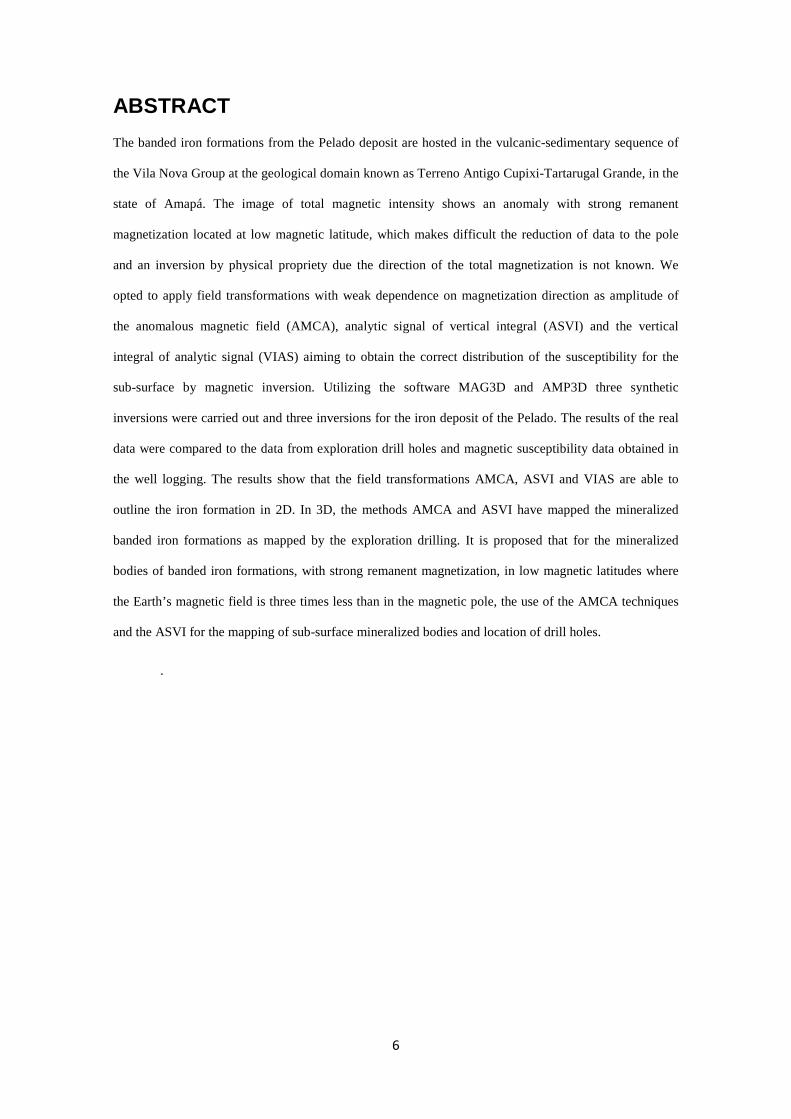
ABSTRACT
The banded iron formations from the Pelado deposit are hosted in the vulcanic-sedimentary sequence of
the Vila Nova Group at the geological domain known as Terreno Antigo Cupixi-Tartarugal Grande, in the
state of Amapá. The image of total magnetic intensity shows an anomaly with strong remanent
magnetization located at low magnetic latitude, which makes difficult the reduction of data to the pole
and an inversion by physical propriety due the direction of the total magnetization is not known. We
opted to apply field transformations with weak dependence on magnetization direction as amplitude of
the anomalous magnetic field (AMCA), analytic signal of vertical integral (ASVI) and the vertical
integral of analytic signal (VIAS) aiming to obtain the correct distribution of the susceptibility for the
sub-surface by magnetic inversion. Utilizing the software MAG3D and AMP3D three synthetic
inversions were carried out and three inversions for the iron deposit of the Pelado. The results of the real
data were compared to the data from exploration drill holes and magnetic susceptibility data obtained in
the well logging. The results show that the field transformations AMCA, ASVI and VIAS are able to
outline the iron formation in 2D. In 3D, the methods AMCA and ASVI have mapped the mineralized
banded iron formations as mapped by the exploration drilling. It is proposed that for the mineralized
bodies of banded iron formations, with strong remanent magnetization, in low magnetic latitudes where
the Earth’s magnetic field is three times less than in the magnetic pole, the use of the AMCA techniques
and the ASVI for the mapping of sub-surface mineralized bodies and location of drill holes.
.
7
SUMÁRIO
1 INTRODUÇÃO ............................................................................................................................ 11
1.1 Objetivos .......................................................................................................................... 12
1.2 Localização e vias de acesso ............................................................................................... 13
1.3 Base de dados .................................................................................................................... 14
1.4 Métodos ............................................................................................................................ 16
1.5 Estrutura da Dissertação ..................................................................................................... 18
2 EMBASAMENTO TEÓRICO ...................................................................................................... 20
2.1 Magnetização e as transformações do campo magnético anômalo .......................................... 20
2.2 Modelagem geofísica e a inversão magnética em 3D ............................................................. 25
2.3 Algoritmos MAG3D e AMP3D ........................................................................................... 34
3 APPLICABILITY OF MAGNETIC INVERSION TO MAP BANDED I RON FORMATIONS AND LOCATE TARGETS IN LOW MAGNETIC LATITUDES WITH STRONG REMANENCE: CASE STUDY OF PELA DO DEPOSIT...................................................................................................................................... 35
3.1 Abstract ............................................................................................................................ 35
3.2 Introduction ....................................................................................................................... 36
3.3 Geological Setting ............................................................................................................. 39
3.4 Geology of Iron Ore Deposits ............................................................................................. 44
3.5 Data base .......................................................................................................................... 47
3.6 Methods ............................................................................................................................ 49
3.7 Synthetic inversion ............................................................................................................ 51
3.8 Results .............................................................................................................................. 55
3.8.1 Processing of magnetic data and characterization of the main targets ...................................... 55
3.8.2 Magnetic lithological characterization ................................................................................. 61
3.8.3 Real data - Inversion .......................................................................................................... 63
3.9 Discussion and conclusions................................................................................................. 73
3.10 Acknowledgement ............................................................................................................. 75
3.11 References ........................................................................................................................ 76
4 DISCUSSÕES E CONCLUSÕES – CONTRIBUIÇÕES DA DISSERTAÇÃO .............................. 79
5 REFERENCIAS BIBLIOGRÁFICAS ........................................................................................... 81
LISTA DE FIGURAS
Figura 1 – Localização do greenstone belt do Grupo Vila Nova em relação as principais cidades do estado do Amapá 13
Figura 2: Localização e mapa geológico regional (CPRM, 2004 e Borghetti et al, 2013) dos depósitos do
Pelado(polígono vermelho) e do Jacu (polígono azul). 14
Figura 3: Fluxograma de processamento do dado magnético terrestre para obtenção dos produtos AMCA, ASVI e
VIAS 17
Figura 4: Perfil magnético de uma fonte magnética cilíndrica sem magnetização induzida (a) e com magnetização
induzida perpendicular a magnetização remanescente (b). 22
8
Figura 5 – Comparação entre as principais transformações de campo utilizadas para a inversão magnética devido a
existência de remanência. (a) campo magnético total, (b) AMCA, (c) ASVI e VIAS (d). Modificado de
Biondo, 2011 25
Figura 6 – Exemplificação do modelo direto. A partir de uma distribuição de susceptibilidade qualquer inserida em
um campo magnético B é possível calcular a anomalia magnética que o corpo terá para uma determinada
altitude z. Modificado de Oldenburg e Li (2007) 26
Exemplo de modelagem direta. A figura (a) é o perfil magnético medido em campo (perfil preto) e o perfil magnético
obtido pelo corpo azul escuro modelado (perfil vermelho). 27
Figura 8 – Exemplificação da inversão geofísica. A partir da anomalia medida, calcula-se a distribuição de
susceptibilidade. Modificado de Oldenburg e Li (2007) 28
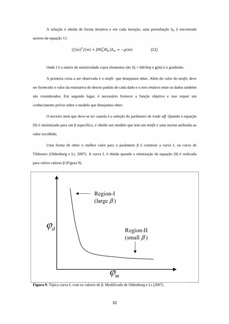
Figura 9 – Típica curva L com os valores de β 32
Figure 10 - Location map of the Vila Nova Group (black polygon) and towns near the research area 38
Figure 11 - Distribution of the geochronological provinces of Amazon Craton. The black polygon indicates the study
area. (Tassinari & Macambira ,2004) 40
Figure 12 - Distribution of Vila Nova Group in the Amapá and Pará state. In this map, it is possible to see the Bacuri
Complex (Uba), Igarapé do Breu (Ubr) and Cupixi (Uc) ultramafic complex. We can see too the Serra do
Navio manganese mine (SN) and the iron ore of the Vila Nova Project (FePVN). Adapted from McReath and
Faraco (2006). The black polygon indicates the study area of Vila Nova Group (Figure 13). 41
Figure 13 - Geological map of the Terreno Antigo Cupixi-Tartarugal Grande with the study area and mineral
occurrences (Borghetti et al, 2013). The red polygon is the Pelado deposit and the blue polygon indicates the
Jacu deposit. 42
Figure 14 - The image of amplitude of analytic signal of the study area. The image enhances the signature of keels
related with the supracrustal (VLG), the magnetic response of Pelado deposit (PD), Cupixi lineament (LC,
white lineament), Bacuri Complex (Uba) and the Amapá Granite (AG). The dotted lines are the main magnetic
lineaments of the region. TACTG indicates the Terreno Antigo Cupixi-Tartarugal Grande. Extracted from
CPRM 2003 and Airborne Survey Rio Araguari (2004) and Airborne Survey Amapá (2006). 43
Figure 15 - Ternary image (R=K,G=Th,B=U) of the Vila Nova Group. The high K is coincident with the Vila Nova
Group (VLG). The dotted lines are represented the main magnetic contacts and lineaments. Data from
Airborne Survey Rio Araguari (2004) and Airborne Survey Amapá (2006). 44
Figure 16 - The geological map of Pelado deposit. Source: Mineração Amapari. 46
Figure 17 - Schematic section (N-S) over the Jacu deposit. 47
Figure 18 - Flowchart of the magnetic ground data processing to obtain the AMCA, ASVI and VIAS products. 50
Figure 19 - Synthetic body in 3D vision. 52
Figure 20 - Grids of synthetic magnetic anomaly with remanence : (a) total magnetic intensity, (b) ASVI, (c) VIAS
and (d) the amplitude of field magnetic anomaly (AMCA). The models 3D was cut in the line profile A-B. 53
Figure 21 - The results of the synthetic inversion with remanent magnetism. (a) TMI inversion, (b) ASVI inversion,
(c) VIAS inversion and (d) AMCA inversion. 54
Figure 22 - Total magnetic intensity (CMA) over the Pelado deposit. It is possible to see a strong magnetic anomaly,
with almost 3000 nT. 55
9
Figure 23 - Amplitude of analytic signal over the Pelado deposit. The numbers represent the depth in meters
calculated by the An-Eul method. The black circle indicates an N-S structure. 56
Figure 24: The ASVI transformation to Pelado deposit. 58
Figure 25: The VIAS transformation to Pelado deposit. 59
Figure 26: The VIAS transformation to Pelado deposit. 60
Figure 27: Magnetic susceptibility of Jacu Deposit. 61
Figure 28: Magnetic susceptibility of Pelado Deposit 62
Figure 27 - Comparison between the magnetic banded iron formations 63
Figure 30:Comparison between the real magnetic data (a) and the anomaly caused by the body modeled (b). The 3D
models were cut in the profile AB 64
Figure 31: Diagonal cut (profile AB) in the susceptibility block showing the NE dip of modeled body. In the figure
we can see a long vertical extension. This is not real 65
Figure 32: Isosurface in a 3D image under the ASVI grid (a) and without it. The colors represent different values of
susceptibility 65
Figure 33: Comparison between the geophysical model (a) and the geological section (b). DH-PID-04. The black
profile in the figure 33a is the values of magnetic susceptibility. The increasing of the SM values is coincident
of the magnetic model 67
Figure 34: Comparison between the geological model obtained by drill holes (the brown polygon) and the isosurfaces
obtained from the geophysical model. The colors in the isosurfaces have the following value: gray: 0.08 SI,
light blue: 0.15 SI, green: 0.3 SI and red: 0.45 SI 68
Figure 35: Comparison between the real magnetic data (a) and the anomaly caused by the body modeled (b). The 3D
models were cut in the profile AB. 68
Figure 36: The 3D susceptibility block from VIAS inversion cut in the profile AB 69
Figure 37: Comparison between the real magnetic data (a) and the anomaly caused by the body modeled (b). The 3D
models were cut in the profile AB 69
Figure 38: Susceptibility block with the model 70
Figure 39: Isosurfaces from the AMCA susceptibility model with the AMCA grid (a) and without its (b) 70
Figure 40: Comparison between the geophysical model (a) and the geological section (b). DH-PID-05. The black
profile in the figure 40a is the values of magnetic susceptibility. In this model the values of magnetic
susceptibility are coincident with the geophysical model 72
Figure 41 - Comparison between the geological model obtained by drill holes (the brown polygon) and the
isosurfaces obtained from the geophysical model. The colors in the isosurfaces have the following value: gray:
0.1 SI, light blue: 0.12 SI, green:0.3 SI and red:0.5 SI 73
LISTA DE TABELAS
Tabela 1: Materiais e dados utilizados na realização do trabalho 15
Tabela 2:Erros obtidos e utilizados para a inversão das transformações de campo AMCA, ASVI e VIAS 18
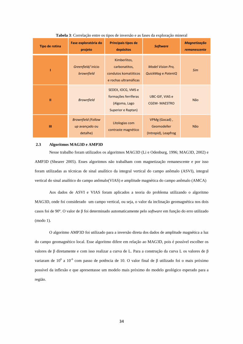
Tabela 3: Correlação entre os tipos de inversão e as fases da exploração mineral 34
Geological reserve and iron ore grades of the main deposits of Vila Nova Group. (Modified from Spier and Filho ,
1999). 46

10
Table 5: Geological reserve and current production of the main iron ore deposit in Vila Nova trend 46
Table 6: The table illustrates the main data used in this research 48
Table 7: Errors used for inversion in AMCA, ASVI and VIAS products. 50
Table 8: Comparison between the results and the three used methods 71
LISTA DE ABREVIATURAS
AMCA – Amplitude Magnética do Campo Anomalo;
AMP3D - Algoritmo para calcular a inversão utilizando dados de amplitude magnética;
ASA – Amplitude do Sinal Analítico;
ASVI – Sinal Analítico da Integral Vertical (Analyitc Signal of Vertical Integration);
CGEM – Center for gravity, Eletric and Magnetic Studies;
CPRM – Companhia de Pesquisa e Recursos Minerais – Serviço Geológico do Brasil;
IOCG – Iron Oxide-Copper-Gold;
MAG3D – Algoritomo para calcualar a inversão utilizando os dados de ASVI e VIAS;
SEDEX – Sedementary Exhalative Deposit;
UBC-GIF: University of British Columbia - Geophysical Inversion Facilities;
VIAS – Integral Vertical do Sinal Analítico (Vertical Integral of Analytic Signal).
11
CAPÍTULO 01
1 INTRODUÇÃO
Dentro do programa de exploração mineral para minério de ferro a magnetometria ocupa um
papel de destaque, principalmente na fase de reconhecimento e seleção de anomalias magnéticas
(Hagemann et al, 2007). Esse destaque é propiciado exclusivamente pelas características magnéticas das
formações ferríferas bandadas (Kerr et al, 1994).
Atualmente as técnicas de interpretação quantitativas e as inversões têm evoluído através dos
anos, porém ainda é complicado obter bons resultados para fontes magnéticas para as quais não se
conhecem a direção de magnetização, ou seja, com a presença de magnetização remanescente (Paine
2001, Shearer 2005). Em regiões de baixa latitude magnética o problema se torna mais critico, uma vez
que os algoritmos de redução ao polo são instáveis e os resultados, a maioria das vezes, não são
confiáveis. Mesmo em regiões com alta latitude magnética a interpretação dos dados magnéticos pode se
tornar uma tarefa árdua quando a direção da magnetização total não é conhecida (Haney et al, 2003).
Para a interpretação e inversão dos dados magnéticos de alvos com magnetização remanescente e
localizados na zona equatorial magnética, pode se aplicar transformações de campo que apresentam
pouca dependência da direção de magnetização, tais como indicado por Shearer (2005) e Paine (2001).
Essas transformações são baseadas na amplitude do sinal analítico (ASA) e vetor do gradiente total do
campo magnético.
Paine (2001) sugere a utilização de duas diferentes transformações: sinal analítico da integral
vertical do campo anômalo (Analytic Signal of Vertical Integration - ASVI) e a integral vertical do sinal
analítico do campo anômalo (Vertical Integration of Analytic Signal - VIAS) para tentar se obter uma
correta distribuição de susceptibilidade em sub-superficie através da inversão magnética enquanto Shearer
(2005) sugere aplicação da amplitude magnética do campo anômalo (AMCA),
Recentemente essas técnicas de inversão foram aplicadas por Biondo (2011) e Santos (2012)
para contornar o problema da remanência durante a inversão geofísica. Biondo (2011) aplica as
transformações anteriormente e a redução ao polo para obter a inversão magnética do complexo alcalino
localizado no estado de Minas Gerais. Santos (2012) utiliza o AMCA para obter a fonte magnética de
12
uma anomalia causada por um depósito de cobre e ouro do tipo Iron-Oxide-Copper-Gold (IOCG)
localizado na região de Carajás, em baixa latitude magnética, com sucesso, inclusive com a validação dos
resultados através de sondagens exploratórias.
Nesse trabalho aplicaram-se as três transformações citadas anteriormente (ASVI, VIAS e
AMCA) na anomalia magnética do depósito de minério de ferro do Pelado, localizado no Greenstone Belt
- Vila Nova, comparar o resultado das três técnicas com os obtidos com as sondagens exploratórias e com
o modelo geológico proposto para a região, e avaliar a qual transformação apresenta o melhor fonte
magnética.
A meta principal desse trabalho é estabelecer a aplicabilidade da teoria da inversão dos dados
magnéticos, com a utilização das três diferentes transformações de campo magnético anômalo de uma
fonte magnética com magnetização remanescente e localizada em baixas latitudes magnética e suas
aplicações na prospecção de depósitos de ferro.
Através da inversão pretende-se determinar a geometria do depósito de formação ferrífera
bandada, e determinar os parâmetros físicos tais como largura, extensão vertical, profundidade do topo e
valores de susceptibilidade recuperados. Todas essas informações serão confrontadas com os dados
geológicos do banco de dados de sondagem exploratória, banco de dados petrofísicos e modelos
geológicos elaborados a partir das sondagens.
1.1 Objetivos
O objetivo principal é testar a aplicabilidade da inversão dos dados magnéticos, utilizando três
diferentes transformações de campo magnético total de uma fonte magnética com magnetização
remanescente e localizada em baixas latitudes magnética e suas aplicações na prospecção de depósitos de
minério de ferro localizados em regiões equatoriais.
Como objetivos específicos propõem-se:
a) Processamento dos dados aerogeofísicos e terrestres para a obtenção de produtos
inerentes a interpretação e entendimento do contexto geológico da região de estudo;
b) Processamento dos dados de susceptibilidade magnética dos alvos Jacu e Pelado para a
caracterização magnética das litologias;
c) Inversão das anomalias magnéticas do depósito do Pelado com a utilização das
transformações de campo magnético total que têm pequena dependência da direção de
13
magnetização tais como amplitude magnética do campo magnético anômalo (AMCA),
sinal analítico da vertical integral (ASVI) e da integral vertical do sinal analítico
(VIAS);
d) Validação e avaliação dos resultados obtidos nas inversões com os resultados das
sondagens exploratórias realizadas na região de estudo;
1.2 Localização e vias de acesso
A região de estudo encontra-se na porção sul do estado Amapá, localizada próxima às cidades de
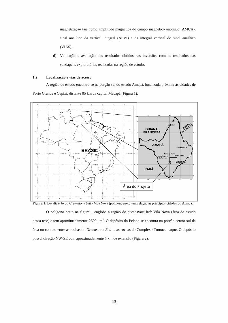
Porto Grande e Cupixi, distante 85 km da capital Macapá (Figura 1).
Figura 1: Localização do Greenstone belt - Vila Nova (polígono preto) em relação às principais cidades do Amapá.
O polígono preto na figura 1 engloba a região do greenstone belt Vila Nova (área de estudo
dessa tese) e tem aproximadamente 2600 km2. O depósito do Pelado se encontra na porção centro-sul da
área no contato entre as rochas do Greenstone Belt e as rochas do Complexo Tumucumaque. O depósito
possui direção NW-SE com aproximadamente 5 km de extensão (Figura 2).
Área do Projeto

14
Figura 2: Localização e mapa geológico regional (CPRM, 2004 e Borghetti et al, 2013) dos depósitos do Pelado(polígono vermelho) e do Jacu (polígono azul).
1.3 Base de dados
Para a realização deste trabalho foi utilizado os dados aerogeofísicos dos projetos Rio Araguari
(CPRM, 2004) e Amapá (CPRM, 2006) disponibilizados pelo Serviço Geológico Brasileiro (CPRM). Os
dois levantamentos foram voados com espaçamentos entre linhas de 500 metros, porém a direção das
linhas de aquisição do projeto Rio Araguari foi de N45Wº e a do projeto Amapá N-S.
A Mineração Amapari AS cedeu os dados de geofísica terrestre sobre o alvo Pelado. As linhas
foram espaçadas em 200 metros e com direção N45ºE (perpendicular as principais feições geológicas) e
espaçamento entre medidas de 0,6 m. Foi utilizado o magnetômetro de vapor de césio da Scintrex –
NAVMAG SM5, na configuração walking mag. Nessa configuração o magnetômetro adquire os dados
automaticamente em sincronia com GPS na frequência de 1 Hz, e um magnetômetro Scintrex ENVIMAG
como magnetômetro base.
Além dos dados de geofísica terrestre a Mineração Amapari SA disponibilizou dados geológicos
de detalhe sobre o alvo Pelado, o banco de dados das sondagens efetuadas na área de trabalho, bem como
os dados de perfilagem geofísica dos furos exploratórios com os dados de susceptibilidade magnética dos
depósitos do Jacu e Pelado.
Para a perfilagem foi utilizado o equipamento KT10 Plus, com a aquisição de três medidas no
mesmo ponto, metro a metro, totalizando 3507 medidas. Desse total, 1299 amostras foram efetuadas no
15
depósito do Pelado, alvo da inversão magnética efetuada nesse trabalho de pesquisa. Destaca-se ainda que
o valor final utilizado representa a média aritmética das três medidas obtidas ponto a ponto.
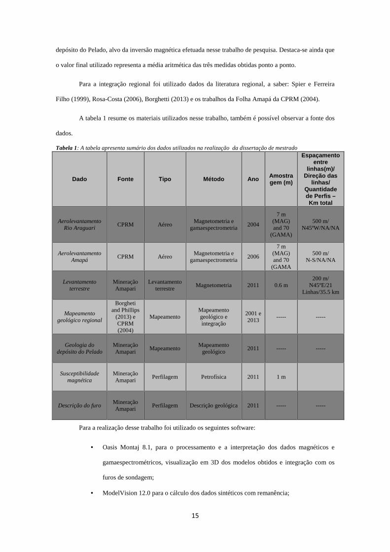
Para a integração regional foi utilizado dados da literatura regional, a saber: Spier e Ferreira
Filho (1999), Rosa-Costa (2006), Borghetti (2013) e os trabalhos da Folha Amapá da CPRM (2004).
A tabela 1 resume os materiais utilizados nesse trabalho, também é possível observar a fonte dos
dados.
Tabela 1: A tabela apresenta sumário dos dados utilizados na realização da dissertação de mestrado
Dado Fonte Tipo Método Ano Amostragem (m)
Espaçamento entre
linhas(m)/ Direção das
linhas/ Quantidade de Perfis – Km total
Aerolevantamento Rio Araguari
CPRM Aéreo Magnetometria e
gamaespectrometria 2004
7 m (MAG) and 70
(GAMA)
500 m/ N45ºW/NA/NA
Aerolevantamento Amapá
CPRM Aéreo Magnetometria e
gamaespectrometria 2006
7 m (MAG) and 70
(GAMA
500 m/ N-S/NA/NA
Levantamento terrestre
Mineração Amapari
Levantamento terrestre
Magnetometria 2011 0.6 m 200 m/
N45ºE/21 Linhas/35.5 km
Mapeamento geológico regional
Borgheti and Phillips
(2013) e CPRM (2004)
Mapeamento Mapeamento geológico e integração
2001 e 2013
----- -----
Geologia do depósito do Pelado
Mineração Amapari
Mapeamento Mapeamento
geológico 2011 ----- -----
Susceptibilidade magnética
Mineração Amapari
Perfilagem Petrofísica 2011 1 m
Descrição do furo Mineração Amapari
Perfilagem Descrição geológica 2011 ----- -----
Para a realização desse trabalho foi utilizado os seguintes software:
• Oasis Montaj 8.1, para o processamento e a interpretação dos dados magnéticos e
gamaespectrométricos, visualização em 3D dos modelos obtidos e integração com os
furos de sondagem;
• ModelVision 12.0 para o cálculo dos dados sintéticos com remanência;
16
• Intrepid 5.0 para processamentos como o Multiscale Edge Detection (MED), junção
dos dados aerogeofísicos e visualização em 3D;
• ArcView 10.01 visando a integração em ambiente SIG dos dados geológicos e
geofísicos;
• CGEM 1.1, software desenvolvido pela Colorado School of Mines, utilizado para a
inversão dos dados de amplitude magnética;
• MAG3D – UBC – 4.0 New Bounds , utilizado para inversão de dados de ASVI e VIAS.
1.4 Métodos
Nesse trabalho de pesquisa utilizaram-se dados de levantamentos aéreos, terrestres e de
perfilagem geofísica. A empresa responsável pela aquisição dos dados aéreos processou os dados
geofísicos e realizou todas as correções necessárias e foram disponibilizados pela CPRM (CPRM, 2004 e
CPRM, 2006). Esses dados foram utilizados para a análise e interpretação da região do trabalho e
adjacências, ou seja, para o entendimento do arcabouço geológico-geofísico regional.
Nos dados magnéticos brutos do magnetometro movel (caixa 1, figura 3) foi realizado o controle
de qualidade e retiradas as medidas espurias (caixa2) e após isso foi aplicado um filtro não linear de 2
fiducias (caixa 3). Já os dados brutos do magnetômetro base (caixa 4) foi aplicada o mesmo controle de
qualidade dos dados (caixa 5) do magnetomêtro móvel e após isso aplicado um filtro passa-baixa de 3
minutos (caixa 6).
A partir do dado do magnetômetro base é aplicada a correção diurna (caixa 7) e é obtido o
campo magnético anomalo (caixa 8), do qual obtemos a AMCA, utiizando o software CGEM – AMP3D
(caixa 9), e exportamos os dados para a inversão (caixa 10).
Para os dados de ASVI, calcula-se a integral vertical do campo anomalo (caixa 11) e depois
calcula-se a amplitude do sinal sinal analítico (caixa 12) do resultado obtido na caixa 14. O resultado
dessa operação é o ASVI e os dados estão prontos para serem exportados (caixa 13).
Já o VIAS, calcula-se a amplitude do sinal analítico do campo anomalo (caixa 14) e depois a
integral vertical, o resultado obtido é o VIAS (caixa 15). O pode se aplicar um filtro passa-alta (caixa 16)
e exporta o dado para a inversão (caixa 17).
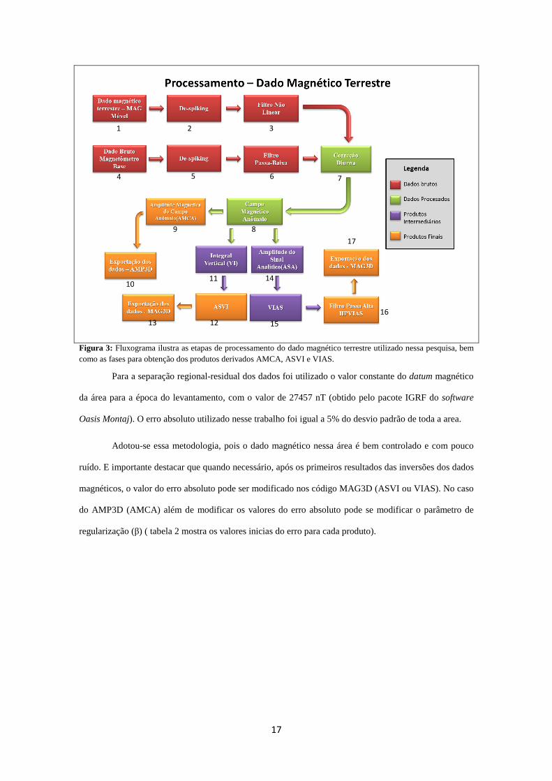
17
Figura 3: Fluxograma ilustra as etapas de processamento do dado magnético terrestre utilizado nessa pesquisa, bem como as fases para obtenção dos produtos derivados AMCA, ASVI e VIAS.
Para a separação regional-residual dos dados foi utilizado o valor constante do datum magnético
da área para a época do levantamento, com o valor de 27457 nT (obtido pelo pacote IGRF do software
Oasis Montaj). O erro absoluto utilizado nesse trabalho foi igual a 5% do desvio padrão de toda a area.
Adotou-se essa metodologia, pois o dado magnético nessa área é bem controlado e com pouco
ruído. E importante destacar que quando necessário, após os primeiros resultados das inversões dos dados
magnéticos, o valor do erro absoluto pode ser modificado nos código MAG3D (ASVI ou VIAS). No caso
do AMP3D (AMCA) além de modificar os valores do erro absoluto pode se modificar o parâmetro de
regularização (β) ( tabela 2 mostra os valores inicias do erro para cada produto).
1 2 3
4 5 6 7
8 9
10 11
12 13
14
15
16
17

18
Tabela 2: Erros obtidos e utilizados para a inversão das transformações de campo AMCA, ASVI e VIAS.
Produto Desvio Padrão (nT) Erro (nT) AMCA 690.06 34.503 ASVI 509.97 24.548 VIAS 719.00 35.950
Antes da inversão com os dados reais foi realizada uma inversão sintética simulando o campo
geomagnético real e o comportamento de cada transformação de campo. A inversão de dados magnéticos
sintéticos é definida como a inversão de fonte magnética controlada onde conhecemos todos os fatores
como geometria, magnetização entre outros. A fonte magnética utilizada nessa fase foi similar ao
depósito do Pelado. Para a inversão dos dados reais foram utilizados os dados topográficos obtidos
através dos levantamentos magnéticos terrestres, sendo que a altura do sensor foi de dois metros acima do
solo e a malha de células para a área foi de 25m x 25m 12.5m (X,Y e Z).
Os dados de susceptibilidade foram tratados estatisticamente com média simples e depois foram
correlacionados pontualmente com dados geológicos extraídos de furos de sondagem disponibilizados
pela Mineração Amapari. Quando era mapeada alguma inconsistência, por exemplo, como alta
susceptibilidade magnética em granitos (nessa região os granitos e ortognaisses presentes no
embasamento não apresentam valores consideráveis de susceptibilidade magnética), efetuou-se uma
revisão dos dados de susceptibilidade. Caso a inconsistência persistisse a descrição geológica do furo era
revista.
Os resultados das inversões foram comparados com a interpretação dos dados geológicos
derivados dos furos de sondagem para a validação ou não do modelo. Os valores de susceptibilidade
magnética recuperados pelas inversões também foram comparados, porém o maior peso foi dado a
“consistência geológica” fornecida pelo modelo.
1.5 Estrutura da Dissertação
Essa dissertação está dividida em cinco capítulos, o primeiro capitulo dedicado a apresentação
do trabalho, objetivos e justificativas, a localização, materiais e métodos.
No segundo capitulo é apresentado o embasamento teórico sobre as técnicas de inversão
magnética 3D e foi baseado no estado da arte sobre o tema em apreço.
O capítulo 3 compreende os resultados principais da pesquisa desenvolvida nessa dissertação
sumarizadas dentro do artigo intitulado Applicability of magnetic inversion to map banded iron

19
formations and locate targets in low magnetic latitudes with strong remanence e submetido ao
periódico Geophysics.
As discussões finais e as contribuições da dissertação de mestrado foram incorporadas dentro do
quarto capitulo. A ultima parte dessa dissertação compreende as referencias bibliográficas.
20
CAPÍTULO 02
2 EMBASAMENTO TEÓRICO
Neste tópico apresenta-se o estado da arte sobre dados magnéticos na presença de magnetismo
remanescente, bem como os conceitos sobre inversão magnética em três dimensões.
2.1 Magnetização e as transformações do campo magnético anômalo
A magnetização de um material é uma quantidade vetorial e é definida matematicamente como a
soma dos momentos dipolares dividido pelo volume de magnetização. Ela pode ser considerada uma
função que varia localmente, e de ponto a ponto (Blakely,1995).
Existem dois tipos de magnetização, a magnetização induzida (Ji) e a magnetização
remanescente (Jr). A magnetização total (J) de um material é definida como a soma dos vetores Ji e Jr
conforme a equação 1 abaixo:
��= ����� + ����� (1)
A magnetização induzida ocorre quando os momentos de dipolo do material estão alinhados na
mesma direção do campo magnético externo, ou seja, o vetor Ji está alinhado na direção do campo
geomagnético local. Quando existe apenas magnetização induzida o vetor J terá direção paralela ao
campo geomagnético (Blakely,1995).
Os minerais magnéticos presentes nas rochas em subsuperficie atuam como pequenos imãs e
adquirem um momento de dipolo. Na ausência de campo magnético externo esses momentos magnéticos
são orientados randomicamente e não existe magnetização (Telford, 1976).
Porém na presença de um campo magnético externo, ou seja, do campo magnético da Terra, os
momentos magnéticos ficam alinhados na direção do campo geomagnético e o material adquire
magnetização. Essa magnetização é proporcional ao campo magnético externo e depende de alguns
fatores como quantidade, composição e tamanhos dos grãos dos minerais magnéticos (Reynolds et al,
1990). A magnetização induzida não é permanente e cessa quando retirado o campo externo.
21
A propriedade física que mede a facilidade com que um material pode ser magnetizado é
conhecida como susceptibilidade magnética (k) e, portanto, podemos definir a magnetização induzida
como:
����� = ���� (2)
onde H é o campo magnético no material e é definida como:
��� = ���� − �� (3)
onde B é o campo magnético externo. É importante notar que as equações 2 e 3, mostram que J não é uma
função linear de k. Nas aplicação da teoria da inversão de dados geofísicos a dados geológicos os valores
de k são frequentemente menores que 1 SI a magnetização induzida é definida como:
����� = ����� (4)
Ao contrário da magnetização induzida, a magnetização remanescente é permanente e é
percebida mesmo na ausência de campo magnético externo (Merril et al, 1996). Os grãos magnéticos da
rocha gravam a direção do campo externo criando uma memória magnética. Como a magnetização total é
a soma das componentes induzida e remanescente, a magnetização total não tem a mesma direção do
campo magnético externo, alterando a forma da anomalia magnética observada na superfície.
A magnetização remanescente é uma função direta do tamanho, quantidade, cristalografia,
arranjo químico dos grãos magnéticos (Reynolds, 1990). É afetada também por fatores geológicos,
tectônicos e pela história térmica dos grãos magnéticos.
Basicamente existem dois tipos de magnetização remanescente: primária e secundária. A
magnetização remanescente primária ocorre durante a formação da rocha e tem a direção do campo
magnético na época da formação ou deposição, e é somada a magnetização induzida. A secundária é
adquirida após a formação e é resultado de processos químicos, térmicos ou pela ação do tempo
(Reynolds, 1990; Moskowitz,2004).
Em termos práticos, a presença de magnetização remanescente muda o formato da anomalia
magnética e a direção da magnetização, desse modo torna-se extremamente difícil a determinação da
fonte magnética a partir dos dados observados, ou seja, o problema inverso.
22
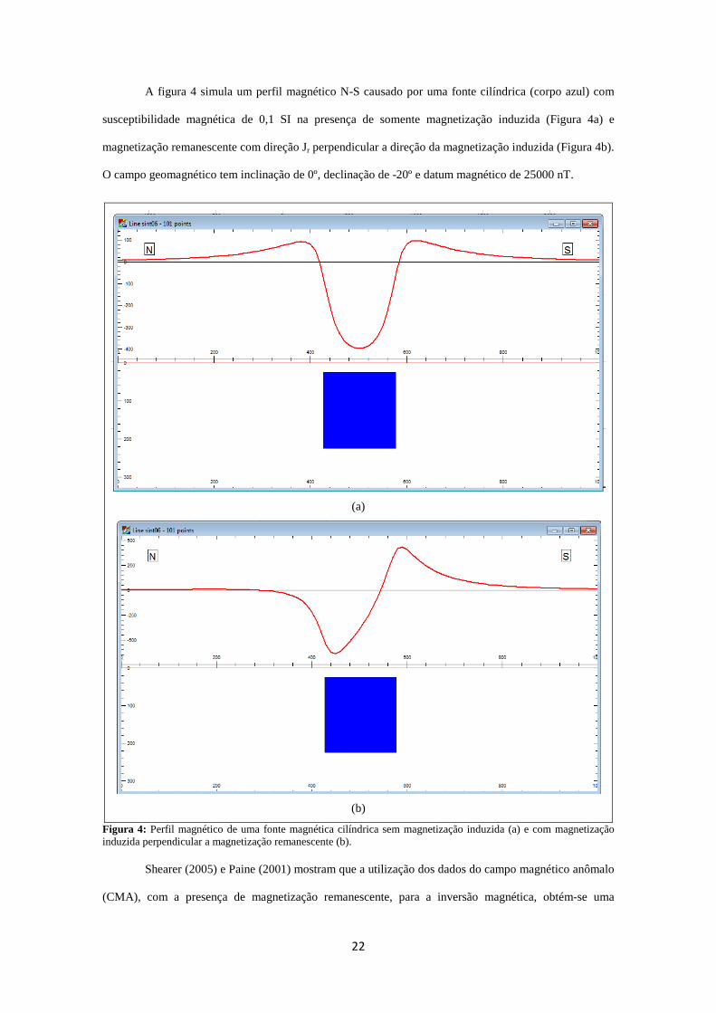
A figura 4 simula um perfil magnético N-S causado por uma fonte cilíndrica (corpo azul) com
susceptibilidade magnética de 0,1 SI na presença de somente magnetização induzida (Figura 4a) e
magnetização remanescente com direção Jr perpendicular a direção da magnetização induzida (Figura 4b).
O campo geomagnético tem inclinação de 0º, declinação de -20º e datum magnético de 25000 nT.
(a)
(b)
Figura 4: Perfil magnético de uma fonte magnética cilíndrica sem magnetização induzida (a) e com magnetização induzida perpendicular a magnetização remanescente (b).
Shearer (2005) e Paine (2001) mostram que a utilização dos dados do campo magnético anômalo
(CMA), com a presença de magnetização remanescente, para a inversão magnética, obtém-se uma
23
distribuição de susceptibilidade magnética totalmente diferente da fonte real e neste caso a utilização
direta, como dado de entrada, do campo magnético anômalo não é viável.
Paine (2001) e Shearer (2005) demostram que o que o melhor caminho é a utilização de
transformações do campo anômalo baseados na amplitude do sinal analítico uma vez que essas
transformações não são afetadas pela presença de magnetização remanescente. Essas transformações são
denominadas de amplitude do campo magnético anômalo (AMCA) sinal analítico da integral vertical do
campo magnético anômalo (ASVI) e a integral vertical do sinal analítico do campo magnético anômalo
(VIAS).
O AMCA é definido através da equação 5 abaixo, onde B é o campo magnético total:
�� = ��������� = ���� + ��� + ��� (5),
Similarmente o gradiente total g do campo anômalo é definido como:
� = ‖∇�‖ = ������� + �����
� + ������ (6)
Como pode ser visto na equação 6 o gradiente e o AMCA são matematicamente similares.
A equação 5 é utilizada diretamente para o cálculo do AMCA enquanto a equação 6 e utilizada
no cálculo do ASVI e VIAS.
A amplitude magnética utiliza a magnitude do campo magnético anômalo vetorial e a magnitude
do vetor gradiente da anomalia magnética. Demonstra-se que a magnitude do vetor gradiente (gradiente
total), frequentemente denominada sinal analítico em 3D, tem pequena dependência da direção de
magnetização.
Essa propriedade é utilizada para a inversão dos dados de amplitude magnética e, dessa forma,
obter a distribuição da magnetização sem conhecimento prévio da direção da mesma.
Nota-se que a magnitude do vetor magnético da anomalia tem propriedade semelhante a
magnitude do vetor gradiente e por isso podemos obter a distribuição da magnitude da magnetização de
modo semelhante com o gradiente total (Shearer, 2005).
Paine (2001) mostra que o VIAS e o ASVI gerados a partir do campo magnético anômalo, geram
respostas magnéticas semelhantes a anomalia observada, se esta fosse gerada apenas por indução
magnética na presença de um campo magnético vertical (inclinação magnética próxima a 90º), com
24
resultados semelhantes a redução ao polo.Segundo o mesmo autor, as duas transformadas ignoram a
presença de magnetização remanescente e incorporam as duas componentes em um simples sinal
coercivo. Entretanto, existe uma série de dificuldades teóricas na utilização dessa técnica. As duas
transformações tem como base o gradiente total e é sabido que esse tipo de campo não é harmonico e por
isso o cálculo do VIAS no domínio de Fourier é invalido. Além disso, a integração vertical do gradiente
total sempre será positiva, enquanto a transformada VIAS não tem restrição quanto a números negativos.
O efeito negativo que é observado na transformada VIAS é a amplificação dos ruídos de baixa frequência
e a redução da taxa de sinal. Para compensar essa perda, os algoritmos de inversão tendem a obter
resultados com fontes mais profundas e com maior extensão vertical.
Como essa metodologia se baseia na amplitude do sinal analítico, a aplicação do cálculo tanto do
ASVI como do VIAS em dados magnéticos terá pouca dependência da magnetização remanescente
presente nos dados, bem como o AMCA (Paine 2001 e Shearer 2005).
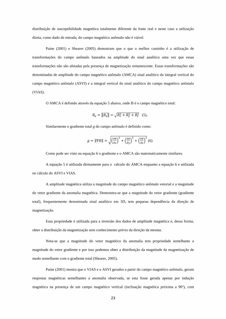
Como exemplo da utilização das transformadas de campo, a figura 5 mostra os produtos obtidos
por Biondo (2011) para o complexo alcalino de Tapira. A figura 5a mostra o campo magnético anômalo
para o complexo, onde se observa forte magnetização remanescente. A figura 5b mostra a AMCA para o
dado de campo magnético anômalo e a figura 5c o ASVI. A figura 5d apresenta o VIAS após a passagem
de um filtro passa alta de 15000 fiduciais.

25
(a)
(b)
(c)
(d)
Figura 5: Comparação entre as principais transformações de campo utilizadas para a inversão magnética devido a existência de remanência. (a) campo magnético total, (b) AMCA, (c) ASVI e VIAS (d). Modificado de Biondo, (2011).
2.2 Modelagem geofísica e a inversão magnética em 3D
A modelagem geofísica pode ser utilizada em diversas fases da exploração mineral tanto nas
fases de greenfield como brownfield, na determinação dos parâmetros geométricos da fonte magnética,
tais como extensão vertical, mergulho, direção do mergulho, etc.
Existem dois diferentes métodos: o primeiro conhecido como modelagem direta e o segundo
como inversão geofísica.
O modelo direto é obtido quando calculamos diretamente a anomalia causada por certa
distribuição de propriedade física, no caso da inversão magnética calcula-se a distribuição de
susceptibilidade magnética (Figura 6).
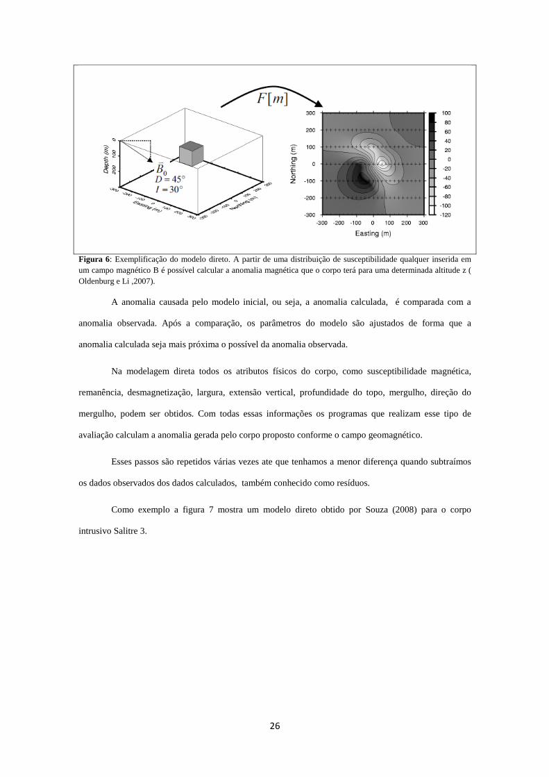
26
Figura 6: Exemplificação do modelo direto. A partir de uma distribuição de susceptibilidade qualquer inserida em um campo magnético B é possível calcular a anomalia magnética que o corpo terá para uma determinada altitude z ( Oldenburg e Li ,2007).
A anomalia causada pelo modelo inicial, ou seja, a anomalia calculada, é comparada com a
anomalia observada. Após a comparação, os parâmetros do modelo são ajustados de forma que a
anomalia calculada seja mais próxima o possível da anomalia observada.
Na modelagem direta todos os atributos físicos do corpo, como susceptibilidade magnética,
remanência, desmagnetização, largura, extensão vertical, profundidade do topo, mergulho, direção do
mergulho, podem ser obtidos. Com todas essas informações os programas que realizam esse tipo de
avaliação calculam a anomalia gerada pelo corpo proposto conforme o campo geomagnético.
Esses passos são repetidos várias vezes ate que tenhamos a menor diferença quando subtraímos
os dados observados dos dados calculados, também conhecido como resíduos.
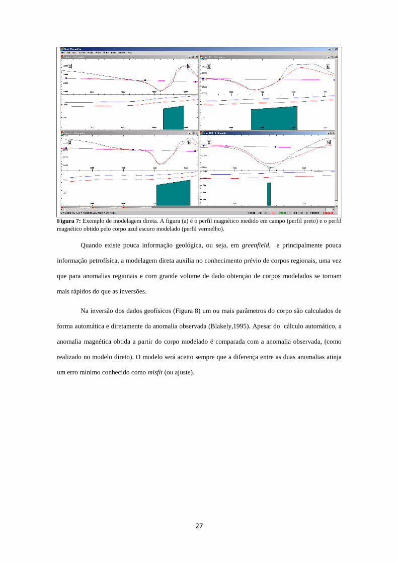
Como exemplo a figura 7 mostra um modelo direto obtido por Souza (2008) para o corpo
intrusivo Salitre 3.
27
Figura 7: Exemplo de modelagem direta. A figura (a) é o perfil magnético medido em campo (perfil preto) e o perfil magnético obtido pelo corpo azul escuro modelado (perfil vermelho).
Quando existe pouca informação geológica, ou seja, em greenfield, e principalmente pouca
informação petrofísica, a modelagem direta auxilia no conhecimento prévio de corpos regionais, uma vez
que para anomalias regionais e com grande volume de dado obtenção de corpos modelados se tornam
mais rápidos do que as inversões.
Na inversão dos dados geofísicos (Figura 8) um ou mais parâmetros do corpo são calculados de
forma automática e diretamente da anomalia observada (Blakely,1995). Apesar do cálculo automático, a
anomalia magnética obtida a partir do corpo modelado é comparada com a anomalia observada, (como
realizado no modelo direto). O modelo será aceito sempre que a diferença entre as duas anomalias atinja
um erro mínimo conhecido como misfit (ou ajuste).
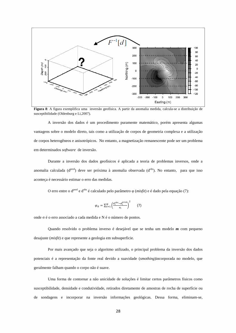
28
Figura 8: A figura exemplifica uma inversão geofísica. A partir da anomalia medida, calcula-se a distribuição de susceptibilidade (Oldenburg e Li,2007).
A inversão dos dados é um procedimento puramente matemático, porém apresenta algumas
vantagens sobre o modelo direto, tais como a utilização de corpos de geometria complexa e a utilização
de corpos heterogêneos e anisotrópicos. No entanto, a magnetização remanescente pode ser um problema
em determinados software de inversão.
Durante a inversão dos dados geofísicos é aplicada a teoria de problemas inversos, onde a
anomalia calculada (dpred) deve ser próxima à anomalia observada (dobs). No entanto, para que isso
aconteça é necessário estimar o erro das medidas.
O erro entre o dpred e dobs é calculado pelo parâmetro φ (misfit) e é dado pela equação (7):
�� = ∑ !�"#$%&�"'()*+" ,�-./0 (7)
onde σ é o erro associado a cada medida e N é o número de pontos.
Quando resolvido o problema inverso é desejável que se tenha um modelo m com pequeno
desajuste (misfit) e que represente a geologia em subsuperficie.
Por mais avançado que seja o algoritmo utilizado, o principal problema da inversão dos dados
potenciais é a representação da fonte real devido a suavidade (smothing)incorporada no modelo, que
geralmente falham quando o corpo não é suave.
Uma forma de contornar a não unicidade de soluções é limitar certos parâmetros físicos como
susceptibilidade, densidade e condutividade, retirados diretamente de amostras de rocha de superfície ou
de sondagens e incorporar na inversão informações geológicas. Dessa forma, eliminam-se,
29
automaticamente os resultados puramente matemáticos e é realizada uma nova abordagem matemática
para a solução do problema inverso.
Pela própria característica da inversão geofísica, esse método é ideal para ser utilizado dentro de
etapas de brownfield, uma vez que existem mais informações geológicas e o modelo obtido pode ser
usado diretamente como auxilio dentro do programa de sondagem exploratória, principalmente quando é
possível utilizar perfilagens geofísicas. No entanto, caso existam informações que possam ser inseridas
dentro das modelagens, a inversão pode ser utilizada em fases de greenfield.
Dentro da exploração mineral pode-se aplicar três métodos diferentes de inversão (Oldenburg e
Pratt, 2007), cada uma é aplicável em diferentes fases da exploração mineral.
Oldenburg e Pratt (2007) dividem da seguinte forma os algoritmos de inversão: inversão discreta
(Tipo I), inversão por propriedade física (Tipo II) e inversão litológica (Tipo III).
Na inversão discreta (Tipo I), o problema inverso é formulado para determinar uma pequena
quantidade de corpos homogêneos, que podem ou não serem distribuídos em 3D.
Geralmente é possível determinar apenas um parâmetro físico (forma dos corpos, propriedade
física, tamanho,etc.) e os corpos são representados por formas geológicas simples ou complexas.
Do ponto de vista matemático o problema inverso é resolvido quando é encontrado um conjunto
de dados que minimiza o misfit dado pela equação (7). Para esse tipo de equação (7), o problema de
ajuste por mínimos quadrados é bem estudado, mas a aplicação direta ainda mostra problemas.
Na inversão do tipo I é utilizada a parametrização simples ou multi-corpos para a modelagem de
discretas alterações nas propriedades de subsuperficie. Geralmente, esses corpos apresentam propriedade
física uniforme, o que lineariza o problema inverso.
A inversão do tipo I é utilizada quando a informação a priori geológica não é aplicada como uma
restrição de soluções. Esse tipo de inversão aplica-se para determinar a estimativa de profundidade de
uma camada, mergulho e valores de susceptibilidade magnética. É considerada uma extensão do modelo
direto, já que esse tipo de algoritmo é utilizado para o refinamento de corpos rígidos e homogêneos
obtidos para anomalias isoladas na modelagem direta.
30
Pelo o que foi dito anteriormente conclui-se que a inversão discreta é ideal para ser utilizada
principalmente na fase de greenfield, justamente por não necessitar muitas informações geológicas e ser
de rápida execução.
Alem da fase de greenfield a inversão do Tipo I tem obtido bons resultados quando aplicado na
prospecção de kimberlitos e carbonatitos. Outra aplicação interessante é modelo geofísico de condutos
komatiiticos para a mineralização de níquel, devido a grande concentração de pirrotita.
Todos esses modelos metalogenéticos são representados por modelos geofísicos de forma
simples (pipe, sills, etc..) e homogêneos, sendo necessário apenas o ajuste das propriedades físicas e sem
grandes variações laterais de propriedade.
O tipo II de inversão magnética é conhecido como inversão por propriedade física e é usado
largamente na indústria da exploração mineral, sendo o método que mais avançou nos últimos anos. O
principal objetivo é encontrar uma distribuição de propriedade em 3D que caracterize a distribuição em
subsuperficie. Em termos numéricos, a subsuperficie é dividida em um grande número de células, cada
uma com um valor para a propriedade física constante e desconhecido.
Nesse tipo de inversão as células devem ser pequenas o suficiente para que o problema não seja
regularizado, ou seja, temos que alcançar o mesmo resultado mesmo se houver diminuição do tamanho
das células. Ao contrário do que acontece na inversão do tipo I, no tipo II, a quantidade de células é maior
que a quantidade de dados e o problema é denominado como indeterminado.
Problemas lineares indeterminados geralmente só apresentam solução quando é incorporada
alguma informação. No caso da inversão do tipo II é introduzido o parâmetro de regularização (β). A
escolha do parâmetro de regularização é crucial uma vez que ele é considerado uma forma primária de
incorporar informações geológicas. Porém, só a determinação do parâmetro de regularização não é
suficiente para que tenha apenas uma solução, visto que infinitas soluções ainda são possíveis. É obvio
que a solução obtida tem que representar o contexto geológico e por isso o modelo necessita da maior
quantidade possível de informação a priori.
Isto é alcançado através da adequada concepção geológica para a função ϕm (função objetivo)
representada pela equação 8.
31
∅2345 = 67 8 9734 − 4�:;5�<= + 6�> 8 9� ?�32&2()@�� A� <= + 6� 8 9� ?�32&2()@�� A� <= +>>6� 8 9� ?2&2()@�� A� <=> (8)
O mref é um modelo de referência, α é o coeficiente que controla a atenuação (smoothing) em
todas as direções em comparação com o background e w é a função de weighting.
Para inversão do tipo II, todos estes parâmetros precisam ser especificados e a complexidade
final do modelo ou seja, função objetivo, depende do conhecimento a priori da geologia ou modelo
geológico.
Os coeficientes α podem ter valores bem diferentes para o mesmo modelo. No caso do modelo
geológico, considerando a Terra como um meio estratificado horizontalmente teremos αx>>αz. A função
weighting é utilizada a partir da informação a priori , principalmente, a partir dos modelos recuperados.
A construção de uma boa função objetivo não é fácil e nem trivial, no entanto, é uma parte
crucial do problema, já que o modelo final e algumas estruturas observadas no modelo final surgirão a
partir dos detalhes de fm. Nesse tipo de abordagem o problema inverso é formulado para minimizar a
função:
∅345 = ∅�345 + B∅2345 (9)
Na equação (9), β é o parâmetro trade-off ou parâmetro de Tikhonov (Tikhonov e Arsenin,
1977), que é ajustado durante a inversão de modo que após a finalização da inversão o modelo final
obtenha o misfit desejado.
Para resolver o problema numericamente, a Terra é dividida em um volume com certa
quantidade de células com valores constantes ,porém desconhecida, de propriedade física. As equações da
função objetivo do modelo e do modelo direto são discretizadas utilizando uma malha de células e a
função objetivo total (soma de todas as células) é dada por:
∅345 = ‖C�3D345 − <EF75‖� + B�C234 −4�:;5�� (10)
Onde Wd e Wn são as matrizes e F é o operador para a modelagem direta. Para a resolução
numérica da equação (10) são aplicadas várias metodologias, porém o método Gauss-Newton é o
procedimento mais aplicado.
32
A solução é obtida de forma iterativa e em cada iteração, uma perturbação δm é encontrada
atraves da equação 11:
3�345G�345 + BC2GC25H2 = −�345 (11)
Onde J é a matriz de sensitividade cujos elementos são Jij = δdi/δmj e g(m) é o gradiente.
A primeira coisa a ser observada é o misfit que desejamos obter. Além do valor do misfit, deve
ser fornecido o valor da estimativa do desvio padrão de cada dado e o erro relativo entre os dados também
são considerados. Em segundo lugar, é necessário fornecer a função objetivo e isso requer um
conhecimento prévio sobre o modelo que desejamos obter.
O terceiro item que deve-se ter cautela é a seleção do parâmetro de trade off. Quando a equação
(9) é minimizada para um β específico, é obtido um modelo que tem um misfit e uma norma atribuída ao
valor escolhido.
Uma forma de obter o melhor valor para o parâmetro β é construir a curva L ou curva de
Tikhonov (Oldenburg e Li, 2007). A curva L é obtida quando a otimização da equação (9) é realizada
para vários valores β (Figura 9).
Figura 9: Típica curva L com os valores de β. Modificado de Oldenburg e Li (2007).
33
A curva de Tikhonov apresenta um formato de L (daí o nome de curva L). Se os erros dos dados
foram estimados corretamente, o melhor valor para β será o ponto de inflexão, se não temos uma
estimativa dos valores dos erros, outros valores de β podem ser escolhidos.
No eixo das ordenadas é possível observar um rápido decaimento do misfit sem o aumento da
norma. Nessa região os dados geofísicos são ajustados. No eixo das odenadas (porção linear), a norma
aumenta com um pequeno misfit, nessa região o erro é ajustado e por isso a melhor relação norma/misfit é
encontrada na inflexão da curva.
A inversão dos dados do tipo II pode ser utilizada onde a anomalia magnética está correlacionada
à própria mineralização, como nos casos de depósitos dos tipos Vulcanic Massive Sulphide (VMS)
,principalmente com pirrotita associada, Iron-Oxide-Copper-Gold (IOCG), sedimentar exalativo
(SEDEX) e formações ferríferas, tanto magnéticas quanto hematíticas.
Devido às características citadas anteriormente, esse tipo de inversão pode ser usada em uma
fase de brownfield visando o auxílio a um programa de sondagem exploratória, já que maiores
informações geológicas são associadas aos resultados geofísicos e quando disponíveis as informações de
campo magnético (não de susceptibilidade magnética) dos furos de sondagem podem ser utilizados para o
refinamento dos resultados.
A inversão litológica (ou tipo III) geralmente é utilizada em fases de brownfield mais avançadas,
durante o follow up de detalhe, já que o ideal é a utilização de dados litológicos, principalmente de furos
de sondagem de susceptibilidade magnética e não dados de campo potencial .
A partir dos dados litológicos, um modelo geológico é obtido e são atribuídos valores de
susceptibilidade a cada litologia, a partir daí a anomalia magnética é calculada e comparada com a
anomalia magnética original.
A tabela 3 resume os métodos de inversão a cada fase de exploração mineral.
34
Tabela 3: Correlação entre os tipos de inversão e as fases da exploração mineral
Tipo de rotina Fase exploratória do
projeto
Principais tipos de
depósitos Software
Magnetização
remanescente
I Greenfield/ início
brownfield
Kimberlitos,
carbonatitos,
condutos komatiiticos
e rochas ultramáficas
Model Vision Pro,
QuickMag e PotentQ Sim
II Brownfield
SEDEX, IOCG, VMS e
formações ferríferas
(Algoma, Lago
Superior e Raptan)
UBC-GIF, VIAS e
CGEM- MAESTRO Não
III
Brownfield (Follow
up avançado ou
detalhe)
Litologias com
contraste magnético
VPMg (Gocad) ,
Geomodeller
(Intrepid), Leapfrog
Não
2.3 Algoritmos MAG3D e AMP3D
Nesse trabalho foram utilizados os algoritmos MAG3D (Li e Odenburg, 1996; MAG3D, 2002) e
AMP3D (Shearer 2005). Esses algoritmos não trabalham com magnetização remanescente e por isso
foram utilizadas as técnicas de sinal analítico da integral vertical do campo anômalo (ASVI), integral
vertical do sinal analítico do campo anômalo(VIAS) e amplitude magnética do campo anômalo (AMCA)
Aos dados de ASVI e VIAS foram aplicados a teoria do problema utilizando o algoritmo
MAG3D, onde foi considerado um campo vertical, ou seja, o valor da inclinação geomagnética nos dois
casos foi de 90º. O valor de β foi determinado automaticamente pelo software em função do erro utilizado
(modo 1).
O algoritmo AMP3D foi utilizado para a inversão direta dos dados de amplitude magnética a luz
do campo geomagnético local. Esse algoritmo difere em relação ao MAG3D, pois é possível escolher os
valores de β diretamente e com isso realizar a curva de L. Para a construção da curva L os valores de β
variaram de 106 a 10-6 com passo de potência de 10. O valor final de β utilizado foi o mais próximo
possível da inflexão e que apresentasse um modelo mais próximo do modelo geológico esperado para a
região.

35
CAPÍTULO 03
3 APPLICABILITY OF MAGNETIC INVERSION TO MAP BANDED I RON FORMATIONS AND LOCATE TARGETS IN LOW MAGNETIC LATITUDES WITH STRONG REMANENCE: CASE STUDY OF PELA DO DEPOSIT
João Paulo Gomes de Souza*, Adalene Moreira Silva*, Catarina Labouré Bemfica Toledo*
Instituto de Geociências – Universidade de Brasília
3.1 Abstract
The banded iron formations from the Pelado deposit are hosted in the vulcanic-sedimentary
sequence of the Vila Nova Group at the geological domain known as Terreno Antigo Cupixi-Tartarugal
Grande, in the state of Amapá. The image of total magnetic intensity shows an anomaly with strong
remanent magnetization located at low magnetic latitude, which makes difficult the reduction of data to
the pole and an inversion by physical propriety due the direction of the total magnetization is not known.
We opted to apply field transformations with weak dependence on magnetization direction as amplitude
of the anomalous magnetic field (AMCA), analytic signal of vertical integral (ASVI) and the vertical
integral of analytic signal (VIAS) aiming to obtain the correct distribution of the susceptibility for the
sub-surface by magnetic inversion. Utilizing the software MAG3D and AMP3D three synthetic
inversions were carried out and three inversions for the iron deposit of the Pelado. The results of the real
data were compared to the data from exploration drill holes and magnetic susceptibility data obtained in
the well logging. The results show that the field transformations AMCA, ASVI and VIAS are able to
outline the iron formation in 2D. In 3D, the methods AMCA and ASVI have mapped the mineralized
banded iron formations as mapped by the exploration drilling. It is proposed that for the mineralized
bodies of banded iron formations, with strong remanent magnetization, in low magnetic latitudes where
the Earth’s magnetic field is three times less than in the magnetic pole, the use of the AMCA techniques
and the ASVI for the mapping of sub-surface mineralized bodies and location of drill holes.
36
3.2 Introduction
The potential methods are the geophysical techniques most applied to the iron ore exploration
and magnetometry is by far the most used method, mainly during the geological reconnaissance
(Hagemann et al, 2007).
The geophysical interpretation of the anomalies caused by iron formations was only limited to
qualitative methods as the amplitude of analytical signal and euler deconvolution (Reid et al, 1990 and
1995). Li and Oldenburg (1996) have developed reliable magnetic inversion algorithms and improved the
quantitative interpretation. However, these algorithms work exclusively with the induced magnetic
anomalies, presenting low remanent magnetization or with remanent magnetization in the same direction
of the inductor field (Paine, 2001).
Rarely do we find in nature banded iron formations presenting only induced magnetization,
being often the presence of remanent magnetization on magnetic signature of iron ore deposits. The
presence of remanent magnetization makes the magnetization direction of the target unknown, becomes
the interpretation and the magnetic inversion more difficult. Even using robust inversion methods, when
the total magnetization is not known, the inversion of this type of data shows a wrong distribution of the
magnetic susceptibility (Paine, 2001;Shearer, 2005).
One of the solutions in this case is to use another geophysical method such as gravity or
electromagnetic methods and applying to the inversion (Miller et al, 2011). When these options are not
available it is possible to use some magnetic field transformation that is not influenced by the remanent
magnetization (Santos et al. 2012) to obtain a feasible 3D model of banded iron formation.
Paine (2001) and Shearer (2005) suggest transformations of the total magnetic intensity (TMI)
based on the amplitude of the analytical signal to overcome the magnetic remanence problem. Shearer
(2005) suggests the use of the amplitude of the anomalous magnetic field (AMCA) and Paine (2001)
suggests the use of two different transformations: analytical signal of vertical integral (ASVI) and vertical
integral of analytic signal (VIAS).
Biondo (2011) uses these transformations and the reduction to the pole (RTP) to solve the
problem of the remanent magnetization, getting good results for the techniques AMCA, ASVI and RTP.
However, for the regions of low magnetic latitudes the RTP algorithms become unstable, not being
37
possible to being used. Therefore we have the alternative of using the ASVI, VIAS and AMCA for
magnetic inversion under these conditions.
Santos (2012) successfully uses amplitude of anomalous magnetic field (AMCA) to obtain the
distribution of susceptibility of magnetic anomaly associated with a deposit of Iron-Oxide-Copper-Gold
(IOCG) located in an equatorial magnetic region.
Paine (2001) shows the transformations ASVI and VIAS are weakly influenced by the remanent
magnetization, and simulates magnetic anomalies with 90º of magnetic inclination, that is, with the
vertical magnetic field and anomalies resulting from only the induced magnetization.
Based on the work of Li and Oldenburg (1996), the academic unit of Earth and Ocean Sciences
of a University of British Columbia, namely UBC – Geophysical Inversion Facility (UBC-GIF)
(https://gif.eos.ubc.ca) it was developed in 2002 the software MAG3D. The aim of the program is to
apply direct modeling and methodologies of magnetic inversion. Usually this software generated realistic
models of magnetic susceptibility distribution in sub-surface in a 3D environment. However, the software
works only with induced magnetization, not being possible to indicate the direction of the remanent
magnetization and then is made necessary to use field transformations such as ASVI and VIAS.
The amplitude of the anomalous magnetic field (AMCA) simulates the induced magnetization
for vertical magnetic field, as the analytical signal of the vertical integral (ASVI) and integral vertical of
analytical signal (VIAS). However, the generation of this product is performed in a different manner,
usually, this data is alike the RTP, being then a work alternative for areas with low magnetic latitude.
For the inversion of the AMCA there were used the algorithm AMP3D (Center for Gravity,
Electrical & Magnetic Studies, 2012; Shearer, 2005) developed and distributed by the CGEM of the
Colorado School of Mines (CSM). The software has generated realistic results for the distribution of the
magnetic susceptibility, even in the presence of a strong remanent magnetization and demagnetization
(Santos et al, 2012). Like the MAG3D it is not possible to input the component of the remaining magnetic
field, being only possible to work with the amplitude of anomalous magnetic field (AMCA).
The goal of this research work is to undertake the magnetic inversion, using the three
transformations: ASVI, VIAS and AMCA of one magnetic source with strong remanent magnetization
and located in the equatorial region (magnetic inclination around 7º and declination around -18.5º) in the
State of Amapá, Northern Brazil (Figure 10). In addition to the problem of the low magnetic latitude and
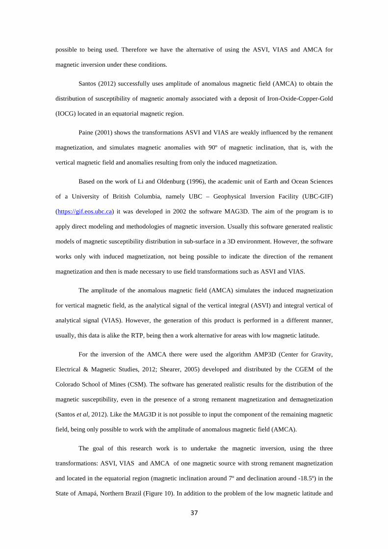
38
strong remanent magnetization, the value of the geomagnetic field is around 25.000 nT, and quite
different from the values, around 60000 nT, observed in the magnetic poles
Figure 10: Location map of the Vila Nova Group (black polygon) and towns near the research area.
The magnetic source at issue is the iron deposit of Pelado that is hosted in iron formations of the
Vila Nova Greenstone Belt (Spier and Filho, 1999). The deposit presents three types of banded iron
formation: siliceous iron formation (IFS), amphibolic iron formation (IFA) and massive iron formation
(IFM), being this last one presenting high iron grades (>55%) and high values of magnetic susceptibility
(>0.5 SI).
Even the massive iron formation the main exploratory target, other types of iron formations
presenting magnetism, and due to the overlapping phenomenon of the magnetic sources it is not possible
to isolate them, being the magnetic source obtained by the inversion of the sum of the three iron
formations.
It is intended then by this work to compare the results by the three techniques, AMCA, ASVI
and VIAS, with the geological model proposed and data of magnetic susceptibility acquired by the
logging of the drill holes and appraise which would be the most effective inversion method given the
conditions (in low magnetic latitudes and strong susceptibility) above and evaluate the respective
application for the prospection of iron ore in equatorial magnetic zones.

39
3.3 Geological Setting
The Amazonian Craton is one of the largest cratonic areas in the world. It underlies the northern
part of South America, and covers an area of about 430.000 km2. The Craton is formed by two
Precambrian shields:Guyana Shield and Brasil Central Shield (or Guaporé Shield), separated by Paleozoic
sedimentary rocks from the Solimões-Amazonas Basin (Almeida et al. 1981). The Craton boundaries are
the Atlantic margin in the north, the Andes Belt in the West and to the East and South, the Neoproterozoic
orogenic Araguaia and Paraguay, respectively.
The Amazonian Craton is subdivided in six different geochronological provinces, defined from
the geochronological standard features, structural trends and particular geological history (Figure 11):
Amazonian Central Province (>2,5 Ga), comprising the Archean nucleus Carajás and Xingu-Iricoumé;
Maroni-Itacaiúnas Province (2.2 – 1,9 Ga); Ventuari-Tapajós Province (1,9 – 1,8 Ga); Rio Negro-Juruena
Province (1,8 – 1,55 Ga); Rondoniana-San Ignácio Province (1,55 Ga – 1,3 Ga) and the Sunsás Province
(1,25 – 1,0 Ga) (Tassinari & Macambira, 2004).
The area of study is located in the northeastern portion of the Amazonian Craton, in the central-
southern part of the Amapá State, and it is part of the Paleoproterozoic province Maroni-Itacaiúnas,
where are found rocks from the vulcanic-sedimentary sequences from the Vila Nova Group (Tassinari
and Macambira,2004, Figure 12). The supracrustal rocks of Vila Nova Group are considered as sequences
of greenstone belt type and are oriented in NW-SE direction, metamorphosed into greenschists to
amphibolites, with ductile-brittle deformation, this deformation generated great shear-zones (Spier and
Ferreira Filho,1999)
In Amapá, the stratigraphy of the Vila Nova Group is characterized, at its base, by a thick pack
of metavulcanic rocks from tholeiitic series, locally komatiites, metamorphosed into greenschist’s facies
to amphibolite (Spier and Ferreira Filho, 1999). On the top, the amphibolites are overlapped by banded
iron formations in oxides and silicates facies, interposed with aluminous-schists presenting lenses of
manganoferous marbles (Serra do Navio Formation). The age suggested by McReath and Faraco (1997)
for these sequences is Paleoproterozoic, around 2.26 ± 0.34 and metamorphism in 1.97 ± 0.51 Ga
(Tassinari, 1997).
40
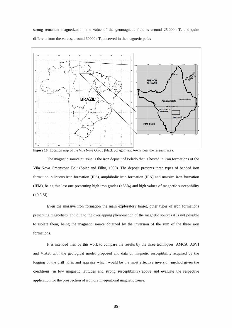
Figure 11: Distribution of the geochronological provinces of Amazon Craton. The black polygon indicates the study area. (Tassinari and Macambira , 2004).
The vulcanic-sedimentary belts composing the Vila Nova Group are hosted in the high grade
terrain of the Guyanense Complex with Archean age, which are constituted of gneiss, migmatites and
41
granulites, (Spier and Ferreira Filho, 1999). All these units have been intensely reworked during the
Transamazonic Orogeny around 2.0 Ga (Tassinari and Macambira, 1999).
The mafic and ultramafic rocks of the Bacuri Complex (Uba, Figure 12) intruded the Archean
basement. This complex are oriented in E-W direction and is constituted of intensely deformed and
metamorphosed rocks in amphibolite facies represented by amphibolites, serpentinites, tremolite and
chromitites (Spier and Ferreira Filho 1999). The Uba hosts important deposits of chromite, being the
second largest Brazilian deposit of chrome (Spier and Ferreira Filho 2001). Isotopic studies (Sm-Nd)
indicate that the intrusion of the Bacuri complex into the continental crust happened around 2.1-2.2 Ga,
approximately at the same time as the volcanism in the Vila Nova Group (Pimentel et al. 2002).
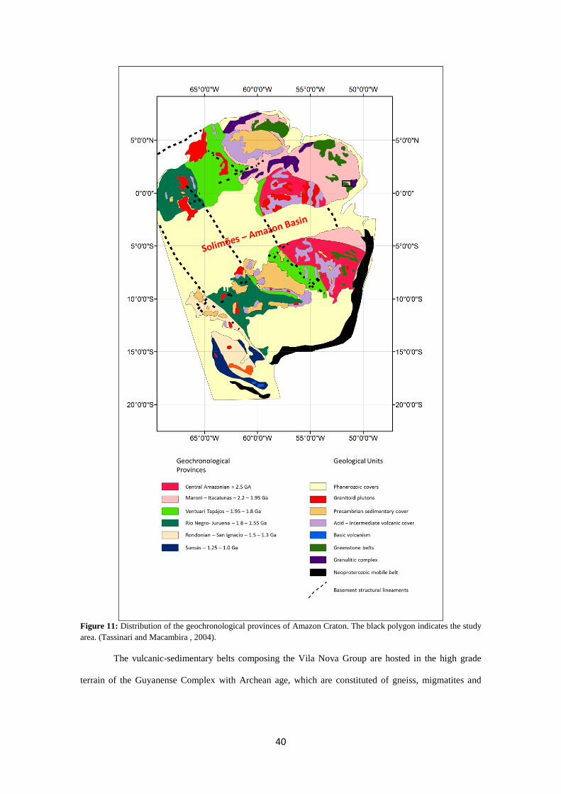
Figure 12: Distribution of Vila Nova Group in the Amapá and Pará state. In this map, it is possible to see the Bacuri Complex (Uba), Igarapé do Breu (Ubr) and Cupixi (Uc) ultramafic complex. We can see too the Serra do Navio manganese mine (SN) and the iron ore of the Vila Nova Project (FePVN). Adapted from McReath and Faraco (2006). The black polygon indicates the study area of Vila Nova Group (Figure 13).
The Pelado deposit is hosted in the vulcanic-sedimentary sequence of the Vila Nova Group in the
geological domain known as Terreno Antigo Cupixi-Tartarugal Grande (Rosa-Costa, 2006 ). In this
region, the Vila Nova Group is distributed in continuous and thin belts presenting direction E-W and NW,
hosted into the Archean gneisses from the Tumucumaque Complex (Figure 13). The basal domain of the
Vila Nova Group is characterized by metabasalts, metadacites and metandesites, presenting the
predominance of the mafic metavulcanic rocks represented by amphibolite and amphibole-schist and
42
amphiboles intercaled with mica schists, marble lenses and graphite-schists. The upper domain is
composed by metasedimentary rocks, with felsic to mafic metavulcanic rocks and chemical - exhalative
subordinated rocks. The detrital metasedimentary rocks present metaconglomerates, quartzites, fuchsite-
quartz schist and micaschists, while those from chemical origin include the banded iron formation
(phylite hematite and schists) and ferruginous quartz (Borghetti et al, 2013). Dating process U-Pb on
zircons from metandesites of this domain indicates the age of 2.17 ±47 Ma for the Vila Nova Group
(Borghetti et al, 2013).
The Amapá and Cigana granites are intrusive in the Vila Nova Group and in the rocks from the
gneiss complex. It shall be highlighted that the Vila Nova Group in this regions is mineralized in Fe and
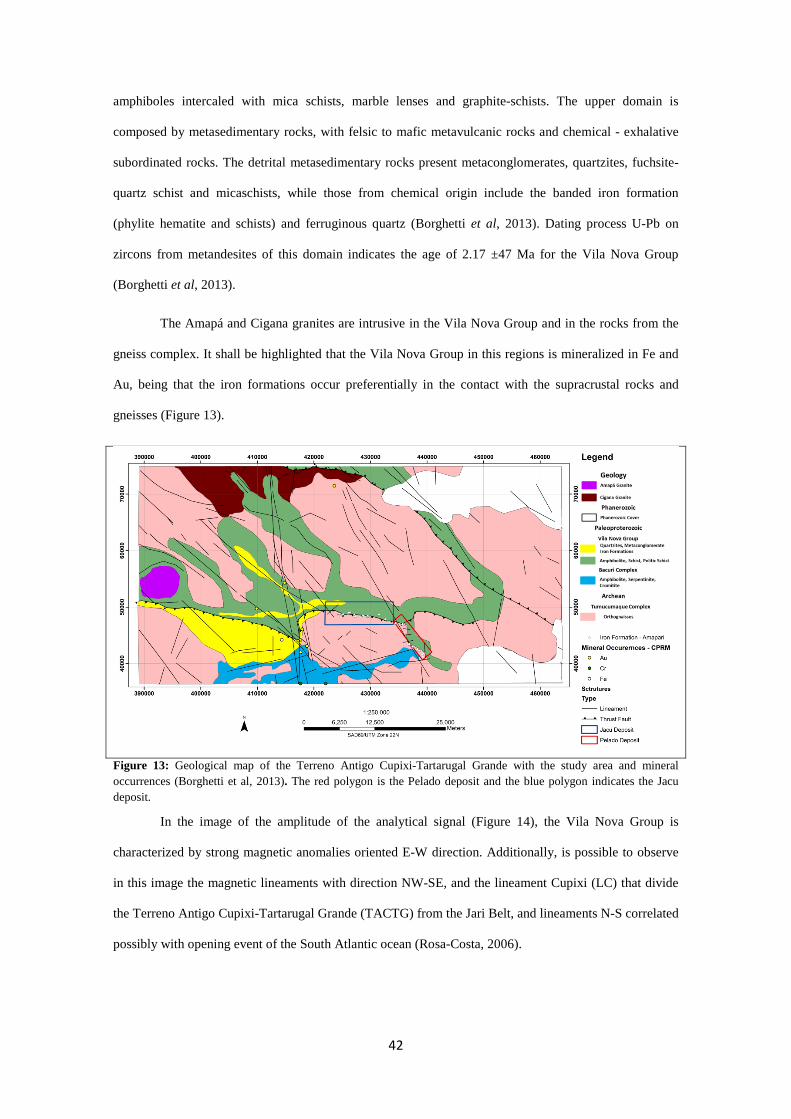
Au, being that the iron formations occur preferentially in the contact with the supracrustal rocks and
gneisses (Figure 13).
Figure 13: Geological map of the Terreno Antigo Cupixi-Tartarugal Grande with the study area and mineral occurrences (Borghetti et al, 2013). The red polygon is the Pelado deposit and the blue polygon indicates the Jacu deposit.
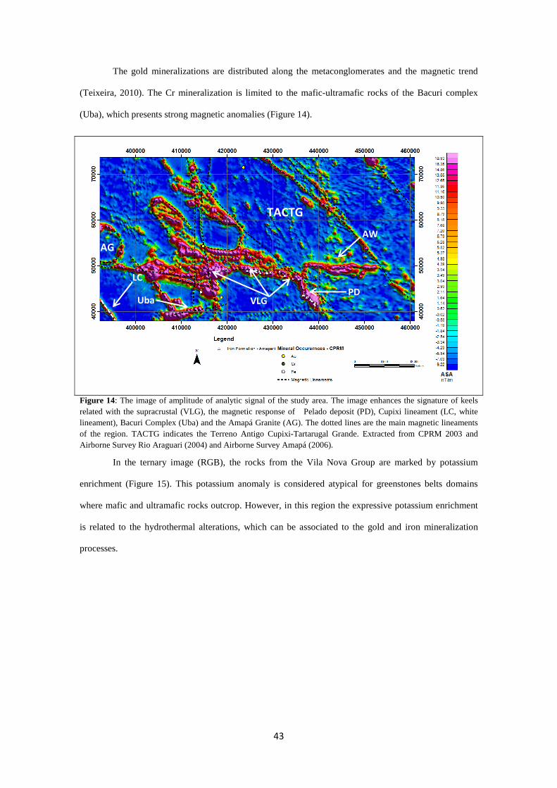
In the image of the amplitude of the analytical signal (Figure 14), the Vila Nova Group is
characterized by strong magnetic anomalies oriented E-W direction. Additionally, is possible to observe
in this image the magnetic lineaments with direction NW-SE, and the lineament Cupixi (LC) that divide
the Terreno Antigo Cupixi-Tartarugal Grande (TACTG) from the Jari Belt, and lineaments N-S correlated
possibly with opening event of the South Atlantic ocean (Rosa-Costa, 2006).
43
The gold mineralizations are distributed along the metaconglomerates and the magnetic trend
(Teixeira, 2010). The Cr mineralization is limited to the mafic-ultramafic rocks of the Bacuri complex
(Uba), which presents strong magnetic anomalies (Figure 14).
Figure 14: The image of amplitude of analytic signal of the study area. The image enhances the signature of keels related with the supracrustal (VLG), the magnetic response of Pelado deposit (PD), Cupixi lineament (LC, white lineament), Bacuri Complex (Uba) and the Amapá Granite (AG). The dotted lines are the main magnetic lineaments of the region. TACTG indicates the Terreno Antigo Cupixi-Tartarugal Grande. Extracted from CPRM 2003 and Airborne Survey Rio Araguari (2004) and Airborne Survey Amapá (2006).
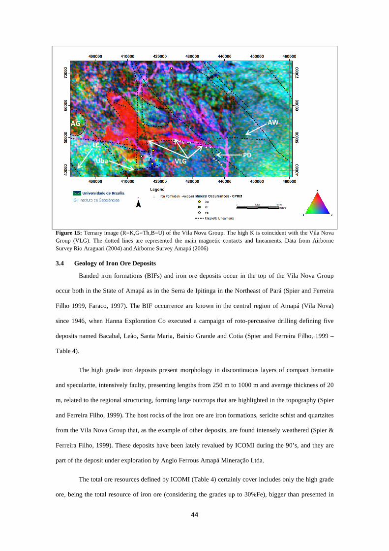
In the ternary image (RGB), the rocks from the Vila Nova Group are marked by potassium
enrichment (Figure 15). This potassium anomaly is considered atypical for greenstones belts domains
where mafic and ultramafic rocks outcrop. However, in this region the expressive potassium enrichment
is related to the hydrothermal alterations, which can be associated to the gold and iron mineralization
processes.
AG
PD VLG
LC
Uba
TACTG
AW
44
Figure 15: Ternary image (R=K,G=Th,B=U) of the Vila Nova Group. The high K is coincident with the Vila Nova Group (VLG). The dotted lines are represented the main magnetic contacts and lineaments. Data from Airborne Survey Rio Araguari (2004) and Airborne Survey Amapá (2006)
3.4 Geology of Iron Ore Deposits
Banded iron formations (BIFs) and iron ore deposits occur in the top of the Vila Nova Group
occur both in the State of Amapá as in the Serra de Ipitinga in the Northeast of Pará (Spier and Ferreira
Filho 1999, Faraco, 1997). The BIF occurrence are known in the central region of Amapá (Vila Nova)
since 1946, when Hanna Exploration Co executed a campaign of roto-percussive drilling defining five
deposits named Bacabal, Leão, Santa Maria, Baixio Grande and Cotia (Spier and Ferreira Filho, 1999 –
Table 4).
The high grade iron deposits present morphology in discontinuous layers of compact hematite
and specularite, intensively faulty, presenting lengths from 250 m to 1000 m and average thickness of 20
m, related to the regional structuring, forming large outcrops that are highlighted in the topography (Spier
and Ferreira Filho, 1999). The host rocks of the iron ore are iron formations, sericite schist and quartzites
from the Vila Nova Group that, as the example of other deposits, are found intensely weathered (Spier &
Ferreira Filho, 1999). These deposits have been lately revalued by ICOMI during the 90’s, and they are
part of the deposit under exploration by Anglo Ferrous Amapá Mineração Ltda.
The total ore resources defined by ICOMI (Table 4) certainly cover includes only the high grade
ore, being the total resource of iron ore (considering the grades up to 30%Fe), bigger than presented in
AG
PD VLG
LC
Uba
AW
45
Table 4. Regional mapping works carried out by ICOMI during the 90’s detected the continuity of the
iron formation towards the northeastern area. However, due to the slight thickness and grade of the
deposits have not been exploited.
The Vila Nova Group has a strong magnetic anomaly and along the magnetic trend there is the
occurrence of iron deposits which have been researched and exploited by Companhia Anglo Ferrous do
Amapá and Mineração Amapari. The litho-structural context of the mineralization suggests the
development of hydrothermal mineralization processes in multiple phases (Teixeira, 2010).
Most of the iron deposits studied by Icomi are hosted in the contacts between the Vila Nova
Group and the basement, the table 5 highlights the major deposits within the magnetic trend of the Vila
Nova Group, in the central portion of the state of Amapá.
In addition to the iron deposits described by Spier and Filho (1999), there have been also mapped
by the Mineração Amapari SA two more iron deposits with grades over 50% located in the contact
between the greenstone belt Vila Nova and the Archean basement, named Jacu and Pelado, subject of the
study and work herein.
The region of these targets have huge weathering layer and it is very common on deposits lack of
outcrops; however is possible to observe blocks of massive iron formation throughout the magnetic trend
of the Vila Nova Group (Figure 13), intercaled with amphibolites, quartzites and pegmatites (Figure 16).
The Jacu deposit presents direction E-W, with 2 km of extension, average thickness of 20 m and
resources of around 6,0 Mt with 50% of cutoff. The Pelado deposit has direction N35ºW, with
approximately 2.5 km of extension and resources around 7 Mt with 50% of cutoff. In both deposits the
mineralized bodies are sub vertical and are hosted in the contact between the metamafic rocks and
granites from the Tumucumaque Complex (Figure 17). The direction of tectonic foliation is E-W at the
Jacu deposit with strong dip (80º-85º) towards south, folding to NW-SE at the eastern portion towards the
Pelado deposit. (Figures 16 and 17)
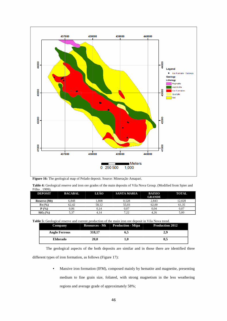
46
Figure 16: The geological map of Pelado deposit. Source: Mineração Amapari.
Table 4: Geological reserve and iron ore grades of the main deposits of Vila Nova Group. (Modified from Spier and Filho , 1999).
DEPOSIT BACABAL LEÃO SANTA MARIA BAIXIO GRANDE
TOTAL
Reserve (Mt) 6,848 1,808 0,528 2,843 12,028 Fe (%) 62,42 58,12 55,03 62,00 61,35 P (%) 0,06 0,14 0,07 0,04 0,07
SiO2 (%) 5,37 4,14 7,22 4,26 5,00
Table 5: Geological reserve and current production of the main iron ore deposit in Vila Nova trend.
Company Resources - Mt Production - Mtpa Production 2012
Anglo Ferrous 318,17 6,5 2,9
Eldorado 20,0 1,0 0,5
The geological aspects of the both deposits are similar and in those there are identified three
different types of iron formation, as follows (Figure 17):
• Massive iron formation (IFM), composed mainly by hematite and magnetite, presenting
medium to fine grain size, foliated, with strong magnetism in the less weathering
regions and average grade of approximately 58%;
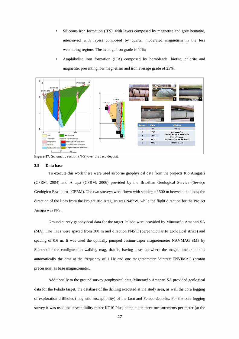
47
• Siliceous iron formation (IFS), with layers composed by magnetite and grey hematite,
interleaved with layers composed by quartz, moderated magnetism in the less
weathering regions. The average iron grade is 40%;
• Amphibolite iron formation (IFA) composed by hornblende, biotite, chlorite and
magnetite, presenting low magnetism and iron average grade of 25%.
Figure 17: Schematic section (N-S) over the Jacu deposit.
3.5 Data base
To execute this work there were used airborne geophysical data from the projects Rio Araguari
(CPRM, 2004) and Amapá (CPRM, 2006) provided by the Brazilian Geological Service (Serviço
Geológico Brasileiro - CPRM). The two surveys were flown with spacing of 500 m between the lines; the
direction of the lines from the Project Rio Araguari was N45ºW, while the flight direction for the Project
Amapá was N-S.
Ground survey geophysical data for the target Pelado were provided by Mineração Amapari SA
(MA). The lines were spaced from 200 m and direction N45ºE (perpendicular to geological strike) and
spacing of 0.6 m. It was used the optically pumped cesium-vapor magnetometer NAVMAG SM5 by
Scintrex in the configuration walking mag, that is, having a set up where the magnetometer obtains
automatically the data at the frequency of 1 Hz and one magnetometer Scintrex ENVIMAG (proton
precession) as base magnetometer.
Additionally to the ground survey geophysical data, Mineração Amapari SA provided geological
data for the Pelado target, the database of the drilling executed at the study area, as well the core logging
of exploration drillholes (magnetic susceptibility) of the Jacu and Pelado deposits. For the core logging
survey it was used the susceptibility meter KT10 Plus, being taken three measurements per meter (at the
48
same point) making the total of 3507 measurements, in this total 1299 samples have been carried out in
the Pelado deposit, target of the magnetic inversion executed in this paper. It shall be emphasized that the
final value used represents the arithmetic average of the three measurements obtained.
For the regional integration it was used the regional geological map (Macapa sheet), 1:250.000,
provided by the Brazilian Geological Service (CPRM, 2004).
Table 6 summarizes the data used in this work, and is also possible to observe the data sources.
Table 6: The table illustrates the main data used in this research.
Data Source Type Method Year Sampling (m)
Line spacing (m)/ Line direction
Rio Araguari Airborne Survey
CPRM Airborne Magnetometric and Radiometric
2004 7 m (MAG)
and 70 (GAMMA)
500 m N45ºW
Amapá Airborne Survey
CPRM Airborne Magnetometric and Radiometric
2006 7 m (MAG)
and 70 (GAMMA
500 m N-S
Ground Surveys
Mineração Amapari
Ground Survey
Magnetometric 2011 0.6 m 200 m
N45ºE/21 lines/35.5 km
Regional geological mapping
Borgheti and Phillips (2013)
Ground mapping
Geological mapping and integration
2013 ----- -----
Geology of Pelado area
Mineração Amapari
Ground mapping
Geological mapping
2011 ----- -----
Magnetic Susceptibility
Mineração Amapari
Core measuring
Petrophysics 2011 1 m
Geological Logging
Mineração Amapari
Logging Geological description
2011 ----- -----
For this work it was used the following software:
• Oasis Montaj 8.1, to processing and interpretation of magnetic and gammaspectometric
data, visualization in 3D of the models generated and integration with the drillholes;
• Model Vision 12.0, to calculate synthetic data with remanence;
• Intrepid 5.0, for more advanced processing such as Multiscale Edge Detection (MED),
merge of the airborne geophysical and visualization in 3D.
49
• ArcView 10.01, for the integration of geophysical and geological data in the GIS
environment;
• CGEM 1.1, software developed by Colorado School of Mines and used for the
inversion of the amplitude of the anomalous magnetic field data;
• MAG3D – UBC – 4.0 New Bounds, used for the data inversion of ASVI and VIAS;
3.6 Methods
In this work there have been used petrophysical data, data from ground survey and airborne
surveys. The airborne data had been delivered already processed and with all corrections done and no
extra data processing was applied to airborne data provided by CPRM. These data have been used for
evaluation and interpretation of the region and surroundings. That is, for the understanding of the regional
structural framework and geological-geophysical structures.
The ground survey data provided have been processed and generated product for the magnetic
inversion. From the raw data of the TMI (from the base and mobile magnetometers) there have been
generated the files containing the data of the AMCA, ASVI and VIAS. Next, the obtained results were
exported in order to be used in the inversions software.
For the AMCA calculation it was used the Maestro software, developed and distributed by the
Colorado School of Mines (CSM), for the calculation of ASVI and VIAS it was used the package
MAGMAP available by the software Oasis Montaj 8.1. The figure 18 shows the flowchart for the
processing of magnetic ground survey.

50
Figure 18: Flowchart of the magnetic ground data processing to obtain the AMCA, ASVI and VIAS products.
For the regional-residual separation it was used a constant value of the magnetic datum at the
epoch of the survey, the datum value was 27457 nT. There shall be emphasized that before the data
exportation it is necessary the measuring the absolute errors of each products. To calculate the error it was
used 5% of the standard deviation of each product (Table 7).
This methodology was adopted, due the magnetic data in this area is highly controlled and
presents little noise, and it is important to highlight that when made necessary, after the first results from
the inversions, the error value can be increased or reduced for the inversion by using the MAG3D (ASVI
or VIAS). In case of the AMP3D (AMCA) there shall be modified the regularization parameter (β) with
the error remaining steady in 5% of the standard deviation. The table 7 presents the initial values of the
error for each product.
Table 7: Errors used for inversion in AMCA, ASVI and VIAS products. Product Standard Deviation (nT) Error (nT) AMCA 690.06 34.503 ASVI 509.97 24.548 VIAS 719.00 35.950
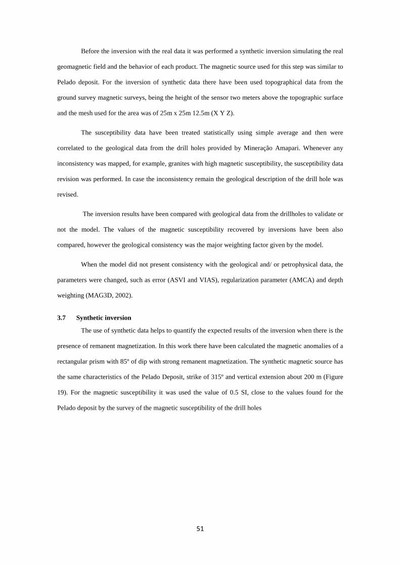
51
Before the inversion with the real data it was performed a synthetic inversion simulating the real
geomagnetic field and the behavior of each product. The magnetic source used for this step was similar to
Pelado deposit. For the inversion of synthetic data there have been used topographical data from the
ground survey magnetic surveys, being the height of the sensor two meters above the topographic surface
and the mesh used for the area was of 25m x 25m 12.5m (X Y Z).
The susceptibility data have been treated statistically using simple average and then were
correlated to the geological data from the drill holes provided by Mineração Amapari. Whenever any
inconsistency was mapped, for example, granites with high magnetic susceptibility, the susceptibility data
revision was performed. In case the inconsistency remain the geological description of the drill hole was
revised.
The inversion results have been compared with geological data from the drillholes to validate or
not the model. The values of the magnetic susceptibility recovered by inversions have been also
compared, however the geological consistency was the major weighting factor given by the model.
When the model did not present consistency with the geological and/ or petrophysical data, the
parameters were changed, such as error (ASVI and VIAS), regularization parameter (AMCA) and depth
weighting (MAG3D, 2002).
3.7 Synthetic inversion
The use of synthetic data helps to quantify the expected results of the inversion when there is the
presence of remanent magnetization. In this work there have been calculated the magnetic anomalies of a
rectangular prism with 85º of dip with strong remanent magnetization. The synthetic magnetic source has
the same characteristics of the Pelado Deposit, strike of 315º and vertical extension about 200 m (Figure
19). For the magnetic susceptibility it was used the value of 0.5 SI, close to the values found for the
Pelado deposit by the survey of the magnetic susceptibility of the drill holes
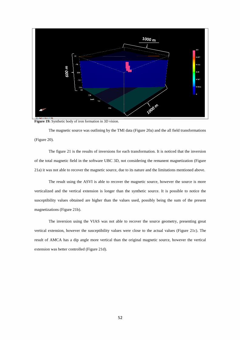
52
Figure 19: Synthetic body of iron formation in 3D vision.
The magnetic source was outlining by the TMI data (Figure 20a) and the all field transformations
(Figure 20).
The figure 21 is the results of inversions for each transformation. It is noticed that the inversion
of the total magnetic field in the software UBC 3D, not considering the remanent magnetization (Figure
21a) it was not able to recover the magnetic source, due to its nature and the limitations mentioned above.
The result using the ASVI is able to recover the magnetic source, however the source is more
verticalized and the vertical extension is longer than the synthetic source. It is possible to notice the
susceptibility values obtained are higher than the values used, possibly being the sum of the present
magnetizations (Figure 21b).
The inversion using the VIAS was not able to recover the source geometry, presenting great
vertical extension, however the susceptibility values were close to the actual values (Figure 21c). The
result of AMCA has a dip angle more vertical than the original magnetic source, however the vertical
extension was better controlled (Figure 21d).
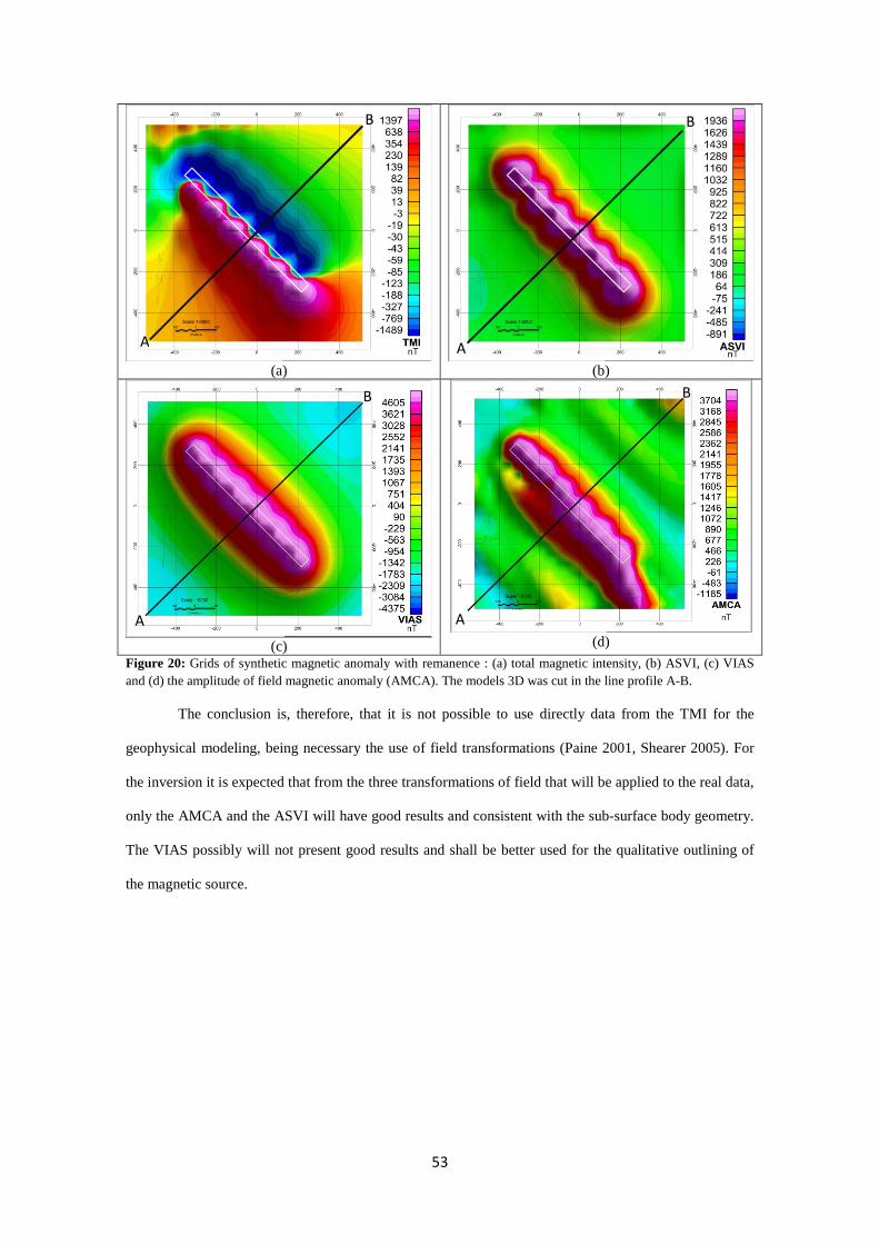
53
(a)
(b)
(c)
(d)
Figure 20: Grids of synthetic magnetic anomaly with remanence : (a) total magnetic intensity, (b) ASVI, (c) VIAS and (d) the amplitude of field magnetic anomaly (AMCA). The models 3D was cut in the line profile A-B.
The conclusion is, therefore, that it is not possible to use directly data from the TMI for the
geophysical modeling, being necessary the use of field transformations (Paine 2001, Shearer 2005). For
the inversion it is expected that from the three transformations of field that will be applied to the real data,
only the AMCA and the ASVI will have good results and consistent with the sub-surface body geometry.
The VIAS possibly will not present good results and shall be better used for the qualitative outlining of
the magnetic source.
A
B
A
B
A
B
A
B

54
(a)
(b)
(c)
Figure 21: The results of the synthetic inversion with remanent magnetism. (a) TMI inversion, (b) ASVI inversion, (c) VIAS inversion and (d) AMCA inversion.
A B
A B
A B
A B
1
0
0.5
0.8
0.42
0
0
0.6
0.3
0
0.1
0.05
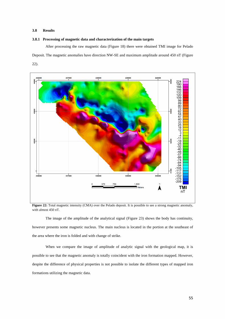
55
3.8 Results
3.8.1 Processing of magnetic data and characterization of the main targets
After processing the raw magnetic data (Figure 18) there were obtained TMI image for Pelado
Deposit. The magnetic anomalies have direction NW-SE and maximum amplitude around 450 nT (Figure
22).
Figure 22: Total magnetic intensity (CMA) over the Pelado deposit. It is possible to see a strong magnetic anomaly, with almost 450 nT.
The image of the amplitude of the analytical signal (Figure 23) shows the body has continuity,
however presents some magnetic nucleus. The main nucleus is located in the portion at the southeast of
the area where the iron is folded and with change of strike.
When we compare the image of amplitude of analytic signal with the geological map, it is
possible to see that the magnetic anomaly is totally coincident with the iron formation mapped. However,
despite the difference of physical properties is not possible to isolate the different types of mapped iron
formations utilizing the magnetic data.
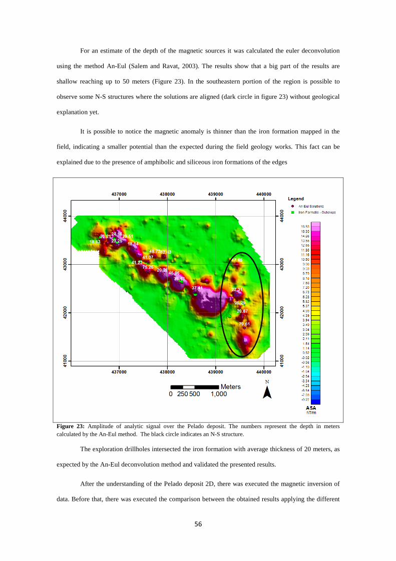
56
For an estimate of the depth of the magnetic sources it was calculated the euler deconvolution
using the method An-Eul (Salem and Ravat, 2003). The results show that a big part of the results are
shallow reaching up to 50 meters (Figure 23). In the southeastern portion of the region is possible to
observe some N-S structures where the solutions are aligned (dark circle in figure 23) without geological
explanation yet.
It is possible to notice the magnetic anomaly is thinner than the iron formation mapped in the
field, indicating a smaller potential than the expected during the field geology works. This fact can be
explained due to the presence of amphibolic and siliceous iron formations of the edges
Figure 23: Amplitude of analytic signal over the Pelado deposit. The numbers represent the depth in meters calculated by the An-Eul method. The black circle indicates an N-S structure.
The exploration drillholes intersected the iron formation with average thickness of 20 meters, as
expected by the An-Eul deconvolution method and validated the presented results.
After the understanding of the Pelado deposit 2D, there was executed the magnetic inversion of
data. Before that, there was executed the comparison between the obtained results applying the different
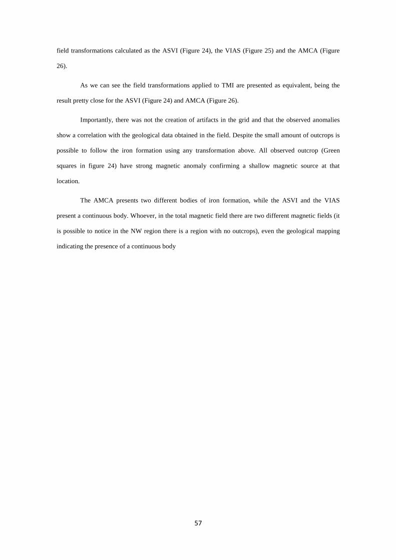
57
field transformations calculated as the ASVI (Figure 24), the VIAS (Figure 25) and the AMCA (Figure
26).
As we can see the field transformations applied to TMI are presented as equivalent, being the
result pretty close for the ASVI (Figure 24) and AMCA (Figure 26).
Importantly, there was not the creation of artifacts in the grid and that the observed anomalies
show a correlation with the geological data obtained in the field. Despite the small amount of outcrops is
possible to follow the iron formation using any transformation above. All observed outcrop (Green
squares in figure 24) have strong magnetic anomaly confirming a shallow magnetic source at that
location.
The AMCA presents two different bodies of iron formation, while the ASVI and the VIAS
present a continuous body. Whoever, in the total magnetic field there are two different magnetic fields (it
is possible to notice in the NW region there is a region with no outcrops), even the geological mapping
indicating the presence of a continuous body
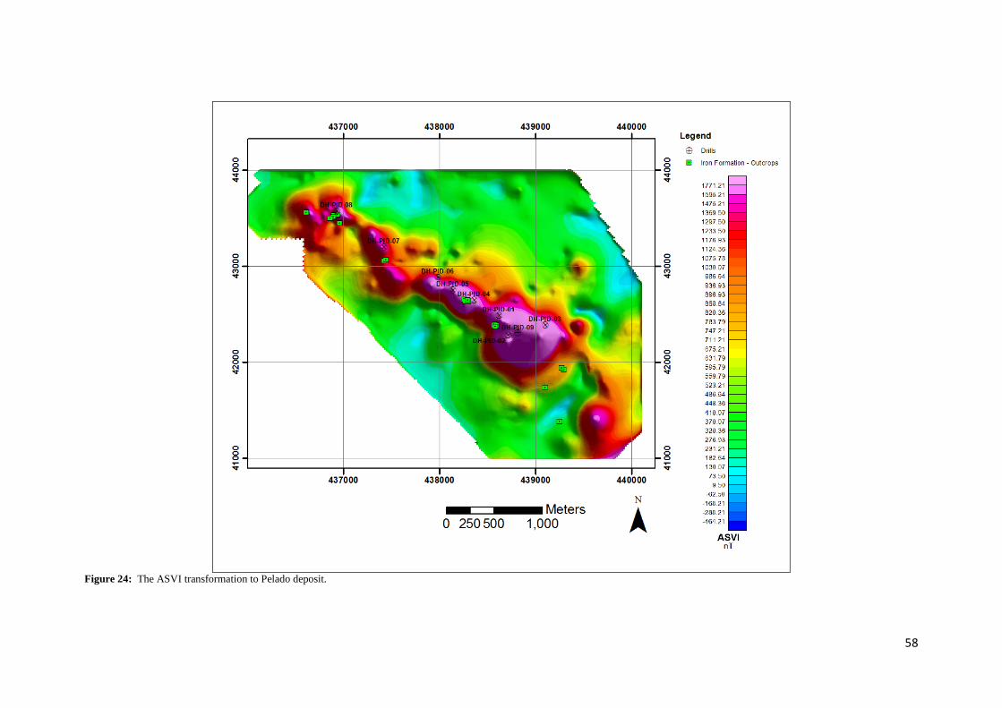
58
Figure 24: The ASVI transformation to Pelado deposit.
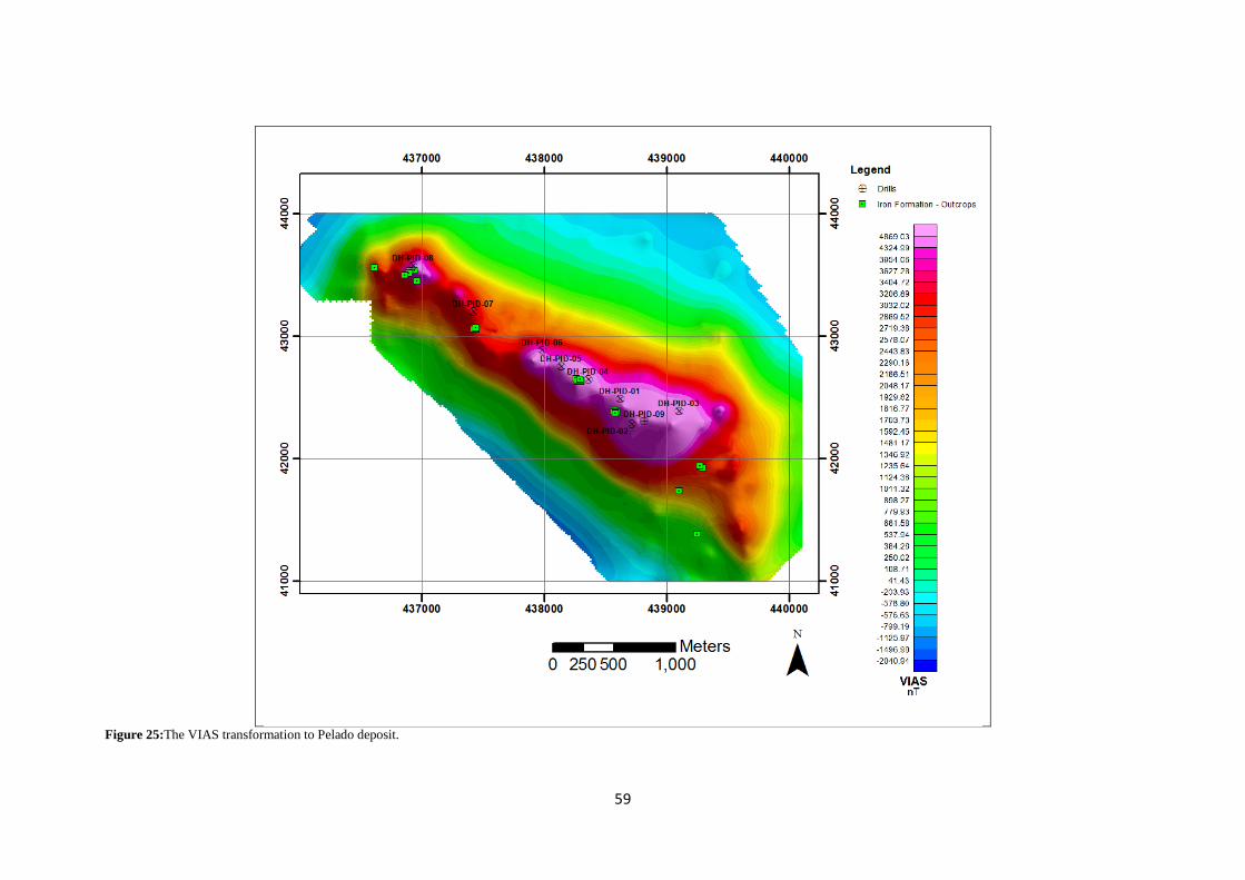
59
Figure 25:The VIAS transformation to Pelado deposit.
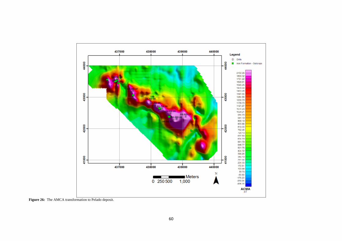
60
Figure 26: The AMCA transformation to Pelado deposit.
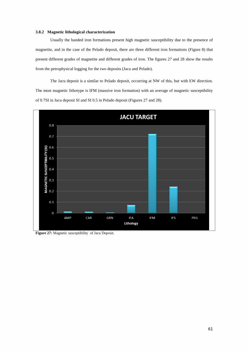
61
3.8.2 Magnetic lithological characterization
Usually the banded iron formations present high magnetic susceptibility due to the presence of
magnetite, and in the case of the Pelado deposit, there are three different iron formations (Figure 8) that
present different grades of magnetite and different grades of iron. The figures 27 and 28 show the results
from the petrophysical logging for the two deposits (Jacu and Pelado).
The Jacu deposit is a similar to Pelado deposit, occurring at NW of this, but with EW direction.
The most magnetic lithotype is IFM (massive iron formation) with an average of magnetic susceptibility
of 0.7SI in Jacu deposit SI and SI 0.5 in Pelado deposit (Figures 27 and 28).
Figure 27: Magnetic susceptibility of Jacu Deposit.

62
Figure 28: Magnetic susceptibility of Pelado Deposit.
The second most magnetic lithotype is the siliceous iron formation with average values of 0.25
SI in Jacu and 0.33 SI in Pelado. In the sequence the IFA (amphibolic iron formation) with values under
0.1 SI in the two deposits. The other lithotypes existing in the region can be considered as not magnetic.
As expected the magnetic anomaly observed for the Pelado deposit (Figure 22) is caused by the
sum of the iron formations IFS+IFA+IFM, being difficult to isolate them in the ground magnetic survey
data.
The difference between the values of magnetic susceptibility between the same lithotype in the
different deposits (Figure 29) is mostly caused by the physical aspect of each rock analyzed. The Pelado
deposit it at lower topographic level than the Jacu deposit and is closer to Piaçaca River, more susceptible
to the variations of the water table and for that presenting higher weathering profile. In additional to the
higher level of weathering, the iron formations found are mostly oxidized at the intervals intersected, and
then the magnetic susceptibility values are lower.
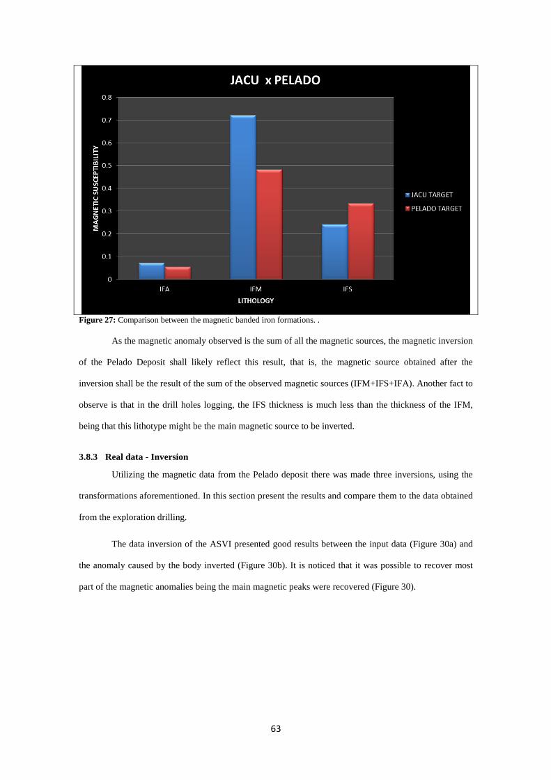
63
Figure 27: Comparison between the magnetic banded iron formations. .
As the magnetic anomaly observed is the sum of all the magnetic sources, the magnetic inversion
of the Pelado Deposit shall likely reflect this result, that is, the magnetic source obtained after the
inversion shall be the result of the sum of the observed magnetic sources (IFM+IFS+IFA). Another fact to
observe is that in the drill holes logging, the IFS thickness is much less than the thickness of the IFM,
being that this lithotype might be the main magnetic source to be inverted.
3.8.3 Real data - Inversion
Utilizing the magnetic data from the Pelado deposit there was made three inversions, using the
transformations aforementioned. In this section present the results and compare them to the data obtained
from the exploration drilling.
The data inversion of the ASVI presented good results between the input data (Figure 30a) and
the anomaly caused by the body inverted (Figure 30b). It is noticed that it was possible to recover most
part of the magnetic anomalies being the main magnetic peaks were recovered (Figure 30).
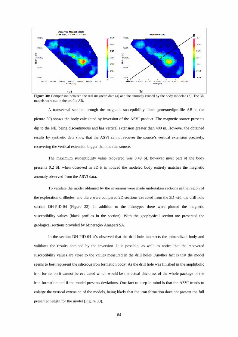
64
(a) (b)
Figure 30: Comparison between the real magnetic data (a) and the anomaly caused by the body modeled (b). The 3D models were cut in the profile AB.
A transversal section through the magnetic susceptibility block generated(profile AB in the
picture 30) shows the body calculated by inversion of the ASVI product. The magnetic source presents
dip to the NE, being discontinuous and has vertical extension greater than 400 m. However the obtained
results by synthetic data show that the ASVI cannot recover the source’s vertical extension precisely,
recovering the vertical extension bigger than the real source.
The maximum susceptibility value recovered was 0.49 SI, however most part of the body
presents 0.2 SI, when observed in 3D it is noticed the modeled body entirely matches the magnetic
anomaly observed from the ASVI data.
To validate the model obtained by the inversion were made undertaken sections in the region of
the exploration drillholes, and there were compared 2D sections extracted from the 3D with the drill hole
section DH-PID-04 (Figure 22). In addition to the lithotypes there were plotted the magnetic
susceptibility values (black profiles in the section). With the geophysical section are presented the
geological sections provided by Mineração Amapari SA.
In the section DH-PID-04 it’s observed that the drill hole intersects the mineralized body and
validates the results obtained by the inversion. It is possible, as well, to notice that the recovered
susceptibility values are close to the values measured in the drill holes. Another fact is that the model
seems to best represent the siliceous iron formation body. As the drill hole was finished in the amphibolic
iron formation it cannot be evaluated which would be the actual thickness of the whole package of the
iron formation and if the model presents deviations. One fact to keep in mind is that the ASVI trends to
enlarge the vertical extension of the models, being likely that the iron formation does not present the full
presented length for the model (Figure 33).
A
B
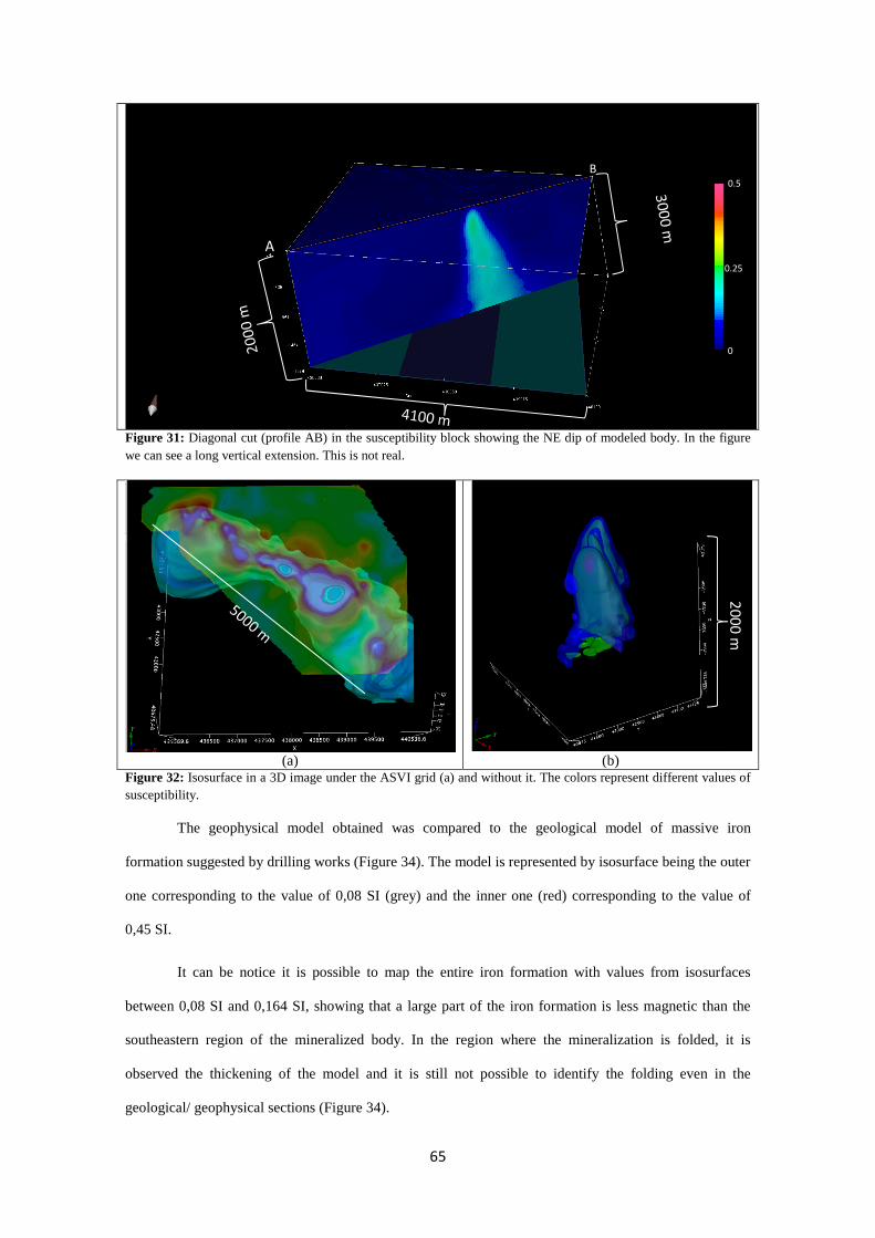
65
Figure 31: Diagonal cut (profile AB) in the susceptibility block showing the NE dip of modeled body. In the figure we can see a long vertical extension. This is not real.
(a)
(b)
Figure 32: Isosurface in a 3D image under the ASVI grid (a) and without it. The colors represent different values of susceptibility.
The geophysical model obtained was compared to the geological model of massive iron
formation suggested by drilling works (Figure 34). The model is represented by isosurface being the outer
one corresponding to the value of 0,08 SI (grey) and the inner one (red) corresponding to the value of
0,45 SI.
It can be notice it is possible to map the entire iron formation with values from isosurfaces
between 0,08 SI and 0,164 SI, showing that a large part of the iron formation is less magnetic than the
southeastern region of the mineralized body. In the region where the mineralization is folded, it is
observed the thickening of the model and it is still not possible to identify the folding even in the
geological/ geophysical sections (Figure 34).
A
B
200
0 m
0.5
0.25
0
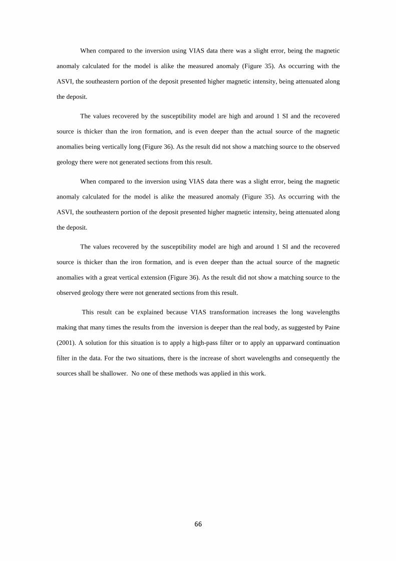
66
When compared to the inversion using VIAS data there was a slight error, being the magnetic
anomaly calculated for the model is alike the measured anomaly (Figure 35). As occurring with the
ASVI, the southeastern portion of the deposit presented higher magnetic intensity, being attenuated along
the deposit.
The values recovered by the susceptibility model are high and around 1 SI and the recovered
source is thicker than the iron formation, and is even deeper than the actual source of the magnetic
anomalies being vertically long (Figure 36). As the result did not show a matching source to the observed
geology there were not generated sections from this result.
When compared to the inversion using VIAS data there was a slight error, being the magnetic
anomaly calculated for the model is alike the measured anomaly (Figure 35). As occurring with the
ASVI, the southeastern portion of the deposit presented higher magnetic intensity, being attenuated along
the deposit.
The values recovered by the susceptibility model are high and around 1 SI and the recovered
source is thicker than the iron formation, and is even deeper than the actual source of the magnetic
anomalies with a great vertical extension (Figure 36). As the result did not show a matching source to the
observed geology there were not generated sections from this result.
This result can be explained because VIAS transformation increases the long wavelengths
making that many times the results from the inversion is deeper than the real body, as suggested by Paine
(2001). A solution for this situation is to apply a high-pass filter or to apply an upparward continuation
filter in the data. For the two situations, there is the increase of short wavelengths and consequently the
sources shall be shallower. No one of these methods was applied in this work.
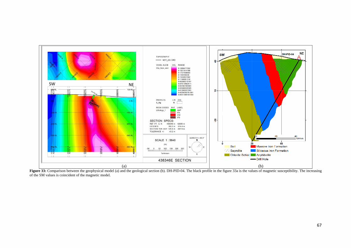
67
(a)
(b)
Figure 33: Comparison between the geophysical model (a) and the geological section (b). DH-PID-04. The black profile in the figure 33a is the values of magnetic susceptibility. The increasing of the SM values is coincident of the magnetic model.
SW NE
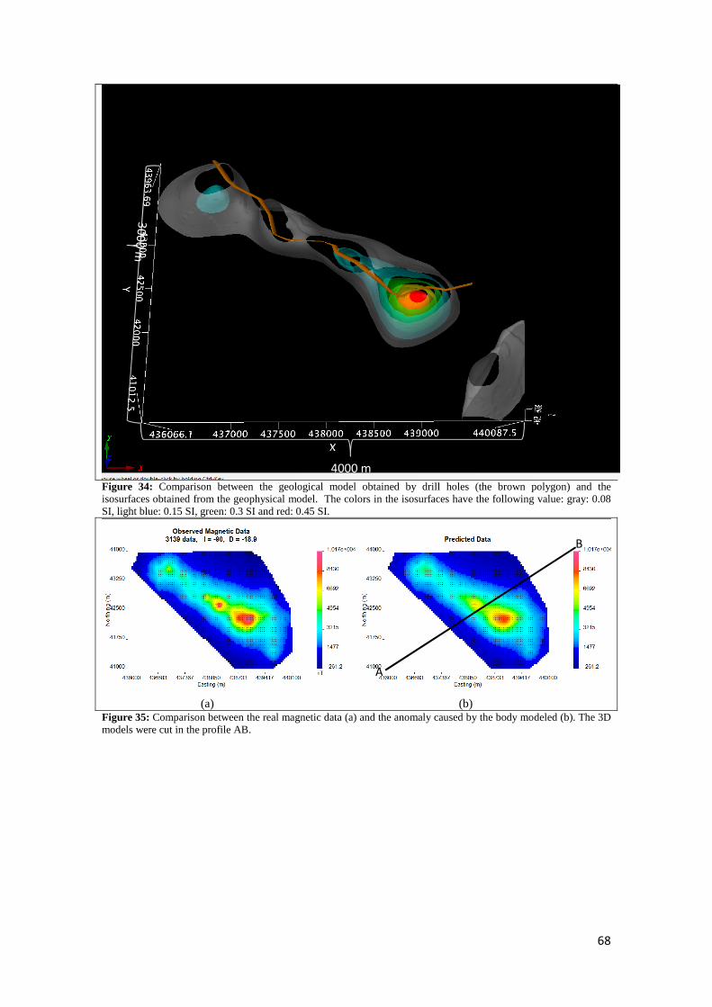
68
Figure 34: Comparison between the geological model obtained by drill holes (the brown polygon) and the isosurfaces obtained from the geophysical model. The colors in the isosurfaces have the following value: gray: 0.08 SI, light blue: 0.15 SI, green: 0.3 SI and red: 0.45 SI.
(a) (b)
Figure 35: Comparison between the real magnetic data (a) and the anomaly caused by the body modeled (b). The 3D models were cut in the profile AB.
4000 m
A
B
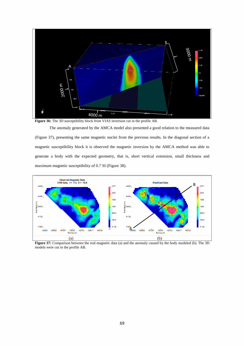
69
Figure 36: The 3D susceptibility block from VIAS inversion cut in the profile AB.
The anomaly generated by the AMCA model also presented a good relation to the measured data
(Figure 37), presenting the same magnetic nuclei from the previous results. In the diagonal section of a
magnetic susceptibility block it is observed the magnetic inversion by the AMCA method was able to
generate a body with the expected geometry, that is, short vertical extension, small thickness and
maximum magnetic susceptibility of 0.7 SI (Figure 38).
(a) (b)
Figure 37: Comparison between the real magnetic data (a) and the anomaly caused by the body modeled (b). The 3D models were cut in the profile AB.
A
B
A
B
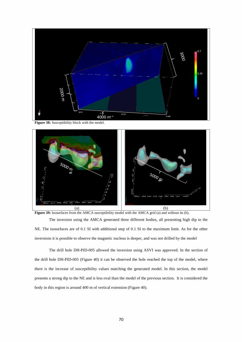
70
Figure 38: Susceptibility block with the model.
(a)
(b)
Figure 39: Isosurfaces from the AMCA susceptibility model with the AMCA grid (a) and without its (b).
The inversion using the AMCA generated three different bodies, all presenting high dip to the
NE. The isosurfaces are of 0.1 SI with additional step of 0.1 SI to the maximum limit. As for the other
inversions it is possible to observe the magnetic nucleus is deeper, and was not drilled by the model
The drill hole DH-PID-005 allowed the inversion using ASVI was approved. In the section of
the drill hole DH-PID-005 (Figure 40) it can be observed the hole reached the top of the model, where
there is the increase of susceptibility values matching the generated model. In this section, the model
presents a strong dip to the NE and is less oval than the model of the previous section. It is considered the
body in this region is around 400 m of vertical extension (Figure 40).
4000 m
0.7
0
0.35
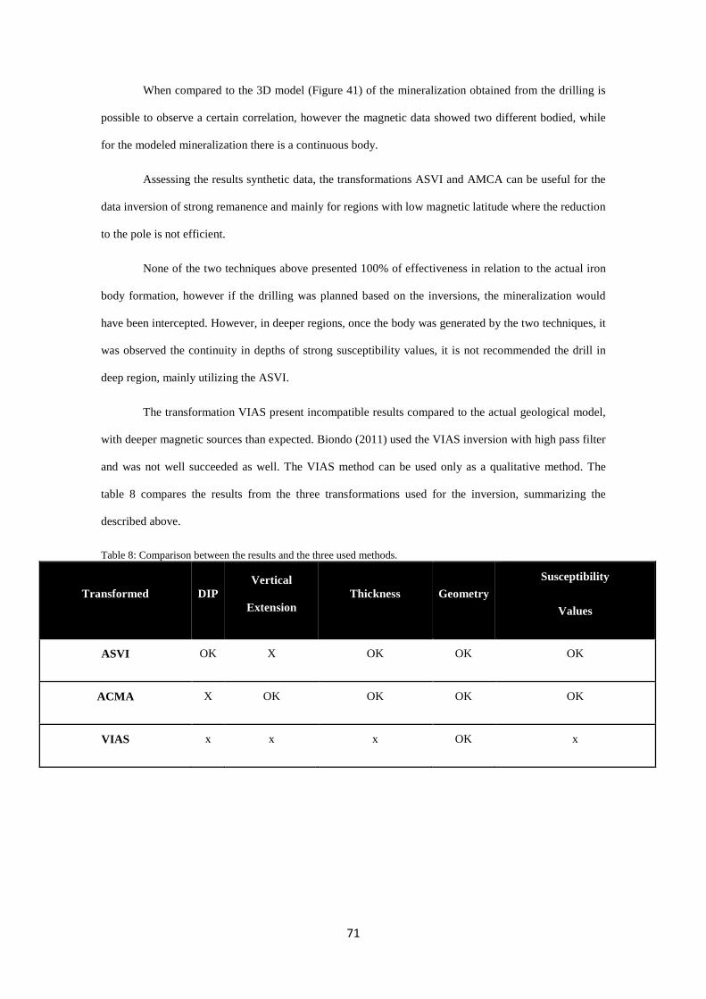
71
When compared to the 3D model (Figure 41) of the mineralization obtained from the drilling is
possible to observe a certain correlation, however the magnetic data showed two different bodied, while
for the modeled mineralization there is a continuous body.
Assessing the results synthetic data, the transformations ASVI and AMCA can be useful for the
data inversion of strong remanence and mainly for regions with low magnetic latitude where the reduction
to the pole is not efficient.
None of the two techniques above presented 100% of effectiveness in relation to the actual iron
body formation, however if the drilling was planned based on the inversions, the mineralization would
have been intercepted. However, in deeper regions, once the body was generated by the two techniques, it
was observed the continuity in depths of strong susceptibility values, it is not recommended the drill in
deep region, mainly utilizing the ASVI.
The transformation VIAS present incompatible results compared to the actual geological model,
with deeper magnetic sources than expected. Biondo (2011) used the VIAS inversion with high pass filter
and was not well succeeded as well. The VIAS method can be used only as a qualitative method. The
table 8 compares the results from the three transformations used for the inversion, summarizing the
described above.
Table 8: Comparison between the results and the three used methods.
Transformed DIP Vertical
Extension Thickness Geometry
Susceptibility
Values
ASVI OK X OK OK OK
ACMA X OK OK OK OK
VIAS x x x OK x
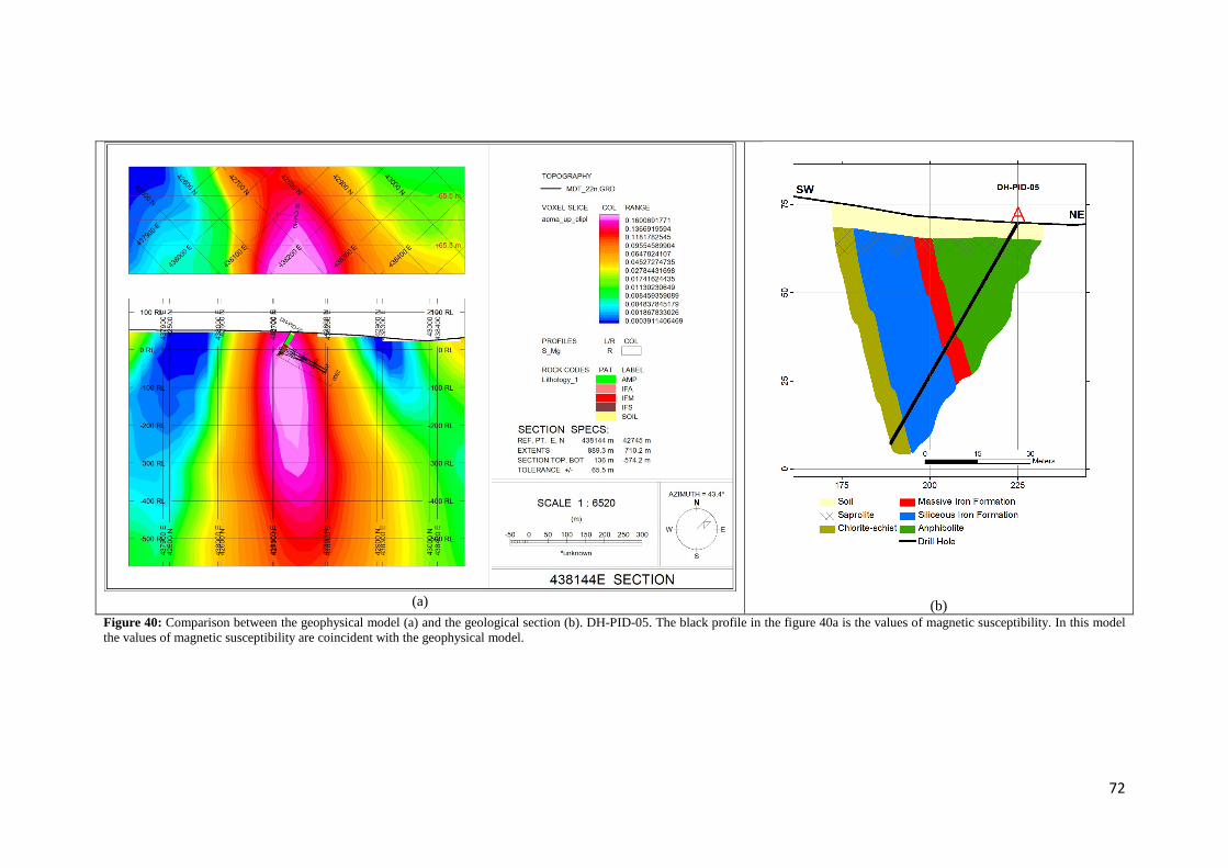
72
(a)
(b) Figure 40: Comparison between the geophysical model (a) and the geological section (b). DH-PID-05. The black profile in the figure 40a is the values of magnetic susceptibility. In this model the values of magnetic susceptibility are coincident with the geophysical model.
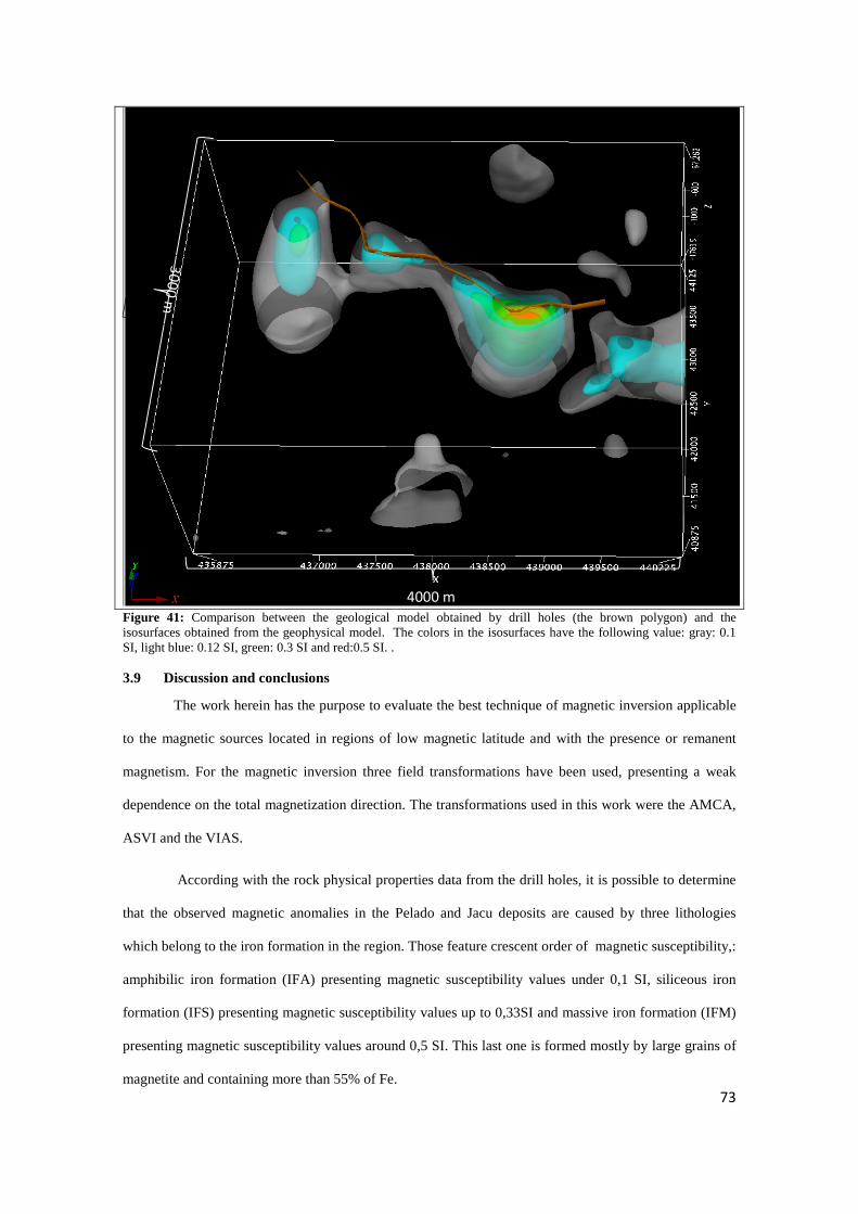
73
Figure 41: Comparison between the geological model obtained by drill holes (the brown polygon) and the isosurfaces obtained from the geophysical model. The colors in the isosurfaces have the following value: gray: 0.1 SI, light blue: 0.12 SI, green: 0.3 SI and red:0.5 SI. .
3.9 Discussion and conclusions
The work herein has the purpose to evaluate the best technique of magnetic inversion applicable
to the magnetic sources located in regions of low magnetic latitude and with the presence or remanent
magnetism. For the magnetic inversion three field transformations have been used, presenting a weak
dependence on the total magnetization direction. The transformations used in this work were the AMCA,
ASVI and the VIAS.
According with the rock physical properties data from the drill holes, it is possible to determine
that the observed magnetic anomalies in the Pelado and Jacu deposits are caused by three lithologies
which belong to the iron formation in the region. Those feature crescent order of magnetic susceptibility,:
amphibilic iron formation (IFA) presenting magnetic susceptibility values under 0,1 SI, siliceous iron
formation (IFS) presenting magnetic susceptibility values up to 0,33SI and massive iron formation (IFM)
presenting magnetic susceptibility values around 0,5 SI. This last one is formed mostly by large grains of
magnetite and containing more than 55% of Fe.
4000 m
74
Despite the IFM being the most magnetic portion of the iron formation, it is the least thick body.
The IFS and IFA iron formations are most significant. The magnetic anomaly is the result of the sum of
the three types, however with a greater contribution of less magnetic portions and greater thickness, like
the IFS and IFA. That shall impact on the generated model, however from the exploratory point of view;
there is no problem once they occur at the same time and location
The euller deconvolution, using the method An-Eul, helped the selection of the acceptable
models since the depth obtained by this methods was in accordance with the outcrops in the area, being
the top of the iron formation around 30 meters deep.
The use of synthetic data as pre-assessment of the data was useful and showed that in a
qualitative manner all the field transformations used in this work where magnetic source, in the presence
of remaining magnetization, and therefore we can conclude that all the three field transformations can be
used during the qualitative interpretation of similar magnetic anomalies.
For the inversion of synthetic magnetic data it was clear the two field transformations ASVI and
AMCA can be used for the inversion of magnetic data presenting remanence. The transformation VIAS
presented deeper results and with a different format from the synthetic source. The direct use of the
anomalous magnetic field data was not able to obtain good results at the data inversion of strong magnetic
remanence, showing the significance of using alternatives when there is this type of magnetization. This
result was expected as seen in Paine (2001) and Shearer (2005).
The application on actual data of the transformations aforementioned obtained the same results
as for the synthetic data. All the transformations were able to outline the iron formation; however VIAS
presents the increase of long wavelengths (Paine, 2001). Is made necessary to use a high pass filter to
improve the results. It can be observed as well that the results from the also ASVI and AMCA are similar
and present slight differences.
In the inversion using ASVI data it was possible to generate a body with the magnetic
susceptibility, shape, dip and thickness compatible with the iron formation intercepted by the exploratory
drilling. However, the vertical extension of the model is not compatible with the geological model. By
comparing the geological sections it is observed there is a good relation between the geological and
geophysical models.
75
The synthetic data using the VIAS did not present good results. The body generated presented as
being deeper and with characteristics of the regional sources with a great vertical extension. This result
was already expected, as presented by the synthetic data. Paine (2001) indicates the VIAS data trend to
present deeper bodies and thicker than the real ones due to the amplification of the noise of low frequency
and the reduction of the signal rate. We can conclude the result herein obtained is in accordance with the
models obtained by other author.
The data inversion using the AMCA was able to recover a magnetic source compatible with the
geological model and the information collected from the drilling and petrophysical data. However it is
observed the dip of the iron formation is more verticalized, being this characteristic a restraint of the
method. Another significant fact is the displacement of the center of the magnetic source, the body
generated is closer to the IFS than to the IFM.
Therefore, we can conclude the transformations AMCA and ASVI can be used for the inversion
of anomalous magnetic field, however there are errors observed related to the dip and the vertical
extension in the generated bodies. From the results it is expected the AMCA is better applicable to
magnetic sources with a strong dip, while the ASVI can be applied to targets with great vertical extension.
The transformation VIAS shall not be used for the inversion, for it did not present any
satisfactory result but the correct plot outlining of the source.
3.10 Acknowledgement
The authors would like to thank the Mineração Amapari for providing the groud survey and
airborne survey data, the geologists Pérsio Mandetta and Carlos Alexandre de Sousa for the support and
technical discussions, A.M Silva would like to thank the National Council of Scientific and Technological
Development (CNPq) for the her fellowship
76
3.11 References
Almeida,F.F.M,.Hasui,Y,.Brito Neves,.B.B,.Fuck,.P.A, 1981. Brazilian structural provinces: an introduction. Earth Sci. Rev., 17:1-29.
Biondo, V, R., 2011 Modelagem geofísica do complexo alcalino de Tapira – MG. Tese de mestrado, IAG/USP, 177p
Bizzi, L.A.; Schobbenhaus,C.; Vidotti, R.M.; Gonçalves, J.H. 2003. Geologia, Tectônica and Recursos Minerais do Brasil, CPRM – Serviço Geological do Brasil, Brasília, 692p.
Blakely.R.J.,1996,Potential Theory in Gravity and Magnetic Applications, Cambridge University Press,USA.
Borghetti, C, Phillip, R. P, Basei, M.A.S,Mandeta,P, 2013, Evolução tectônica do complexo vila nova na região do Cupixi, Porto Grande, Amapá, XIV Simpósio Brasileiro de Estudos Tectonicos – VII International Simposium of Tectonics.
Center for Gravity, Electrical & Magnetic Studies, 2012, AMP3D software package for magnetic amplitude inversion: Colorado School of Mines, http://geophysics.mines.edu/cgem/software.html, accessed 31 March 2012.
CPRM - Serviço Geológico Do Brasil. Carta Geológica do Brasil ao Milionésimo: Sistema de Informações Geográficas-SIG. Folha NA.22 – Macapá. Escala 1:1.000.000. Brasília: CPRM. 2004. 1 CD-ROM. Programa Geologia do Brasil.
CPRM – Serviço Geológico do Brasil.2004. Programa Geologia do Brasil, Projeto Aerogeofísico Rio Araguari, Relatório Final do Levantamento e Processamento dos Dados Magnetométricos e Gamaespectrométricos,Volume I, Texto Técnico, Lasa Engenharia e Prospecções S/A,136p.
CPRM – Serviço Geológico do Brasil.2006. Programa Geologia do Brasil, Projeto Aerogeofísico Amapá, Relatório Final do Levantamento e Processamento dos Dados Magnetométricos e Gamaespectrométricos,Volume I, Texto Tecnico, Lasa Engenharia e Prospecções S/A, Prospectors Aerolevantamentos e Sistemas,272p
Dampney, C. N. G., 1969, The equivalent source technique: Geophysics, 34, 39–53.
Faraco, M.T.L. 1997. Evolução Petroquímico-Metalogenética das Rochas e Mineralizações Associadas à Suíte Vila Nova na Serra do Ipitinga (NW do Pará). Belém, Universidade Federal do Pará. Centro de Geociências. Tese de Doutorado em Geoquímica e Petrologia. p.196p.
Haney, M., C. Johnston, Y. Li, and M. Nabighian, 2003, Envelopes of 2D and 3D magnetic data and their relationship to the analytic signal: Preliminary results: 73rd Annual International Meeting, SEG,Expanded Abstracts, 596–599.
Hagemann.S, Dalstra, H. I. ,Hodkiewicz, P.,Flis, M.,Thorne, W.McCuaig, C.,2007 Recent Advances in BIF-related Iron Ore Models and Exploration Strategies,Proceedings of Exploration 07: Fifth Decennial International Conference on Mineral Exploration edited by B. Milkereit, 2007, p. 811-821
Hrouda.F,Chlupacova.M,Chadima.M,2009, The Use of Magnetic Susceptibility of Rocks in Geological Exploration,TerraPlus, Brno, Czech Republic
Jacobsen, B. H., 1987, A case for upward continuation as a standard separation filter for potential field maps: Geophysics, v. 52, p. 1138-1148.
77
Kerr, T.L., O’Sullivan, A.P., Podmore, D.C., Turner, R., Waters, P.,1994, Geophysics and iron ore exploration: examples from the Jimblebar and Shay Gap-Yarrie Regions, Western Australia, in Geophysical Signatures of Western Australian Mineral Deposits, Geology and Geophysics Department (Key Centre) & UWA Extension, The University of Western Australia, Publication No. 26, 355-367.
Li, Y., and Oldenburg, D. W. 1996, 3-D inversion of magnetic data: Geophysics, v. 61, no. 2, p.394-408.
Li, Y., S. E. Shearer, M. M. Haney, and N. Dannemiller, 2010, Comprehensive approaches to 3D inversion of magnetic data affected by remanent magnetization: Geophysics, 75, no. 1, L1–L11.
MAG3D. A program library for forward modelling and inversion of agnetic data over 3D structures, version 3.1, 2002. Developed under the consortium research project Joint/Cooperative Inversion of Geophysical and Geological Data, UBC-Geophysical Inversion Facility, Department of Earth and Ocean Sciences, University of British Columbia, Vancouver, British Columbia. 2002.
Matos, A.A.; Spier, C.A.; Soares, J.W. 1992. Deposits de Cromita da Região do Rio Vila Nova, Estado do Amapá. In: SBG, Congresso Brasileiro de Geologia, 37, São Paulo, Anais , 246-247.
Miller, R. and Dransfield, M.,2011 -Airborne Gravity Gradiometry and Magnetics in the Search for Economic Iron Ore Deposits: in Proceedings, Iron Ore 2011 Conference, 11-13 July 2011, Perth, Western Australia,The Australasian Institute of Mining and Metallurgy, Melbourne,pp. 109-116
McReath, I. & Faraco, M.T.L. 1997. Sm/Nd and Rb/Sr systems in part of the Vila Nova metamorphic suite, northern Brazil. In: South American Symposium on Isotope Geology, 1, Campos do Jordão, 1997. Extended Abstracts, p.194-196.
Oldenburg.D.W and Pratt.D.A,2007, Geophysical Inversion for Mineral Exploration: a decade of Progress in Theory and Practice, Proceedings of Exploration 07: 5th Decennial International Conference on Mineral Exploration,p.61-95
Oldenburg.D.W and Li.Y,2007,Inversion for Applied Geophysics:A Tuturial,EOS,Vancouver Canadá
Paine, J; Haederle, M; Fils, 2001 M. Using transformed TMI data to invert for remanently magnetized bodies. Exploration Geophysics, vol. 31, n. 3-4, p. 238-242. Reid Ab. 1995. Euler deconvolution: past, present and future – a review. In Anais 65th Annual International Meeting 65th Society of Exploration Geophysicists, 272–273, Houston, Texas.
Pimentel M.M., Spier C. A., Filho C. F. F. 2002. Estudo Sm-Nd do complexo máfico-ultramáfico Bacuri, Amapá: Idade da intrusão, metamorfismo e natureza do magma original. Rev. Bras. Geoc,. 32(3):371-376
Reid Ab, Allsop JM, Granser H, Millett AJ & Somerton Iw.1990. Magnetic interpretation in three dimensions using Euler deconvolution.Geophysics, 55: 80–91.
Rosa-Costa, L. T.,2006, Geocronologia 207Pb/206Pb, Sm-Nd, U-Th-Pb and 40Ar-39Ar do Segmento Sudeste do Escudo das Guianas: Evolução Crustal and Termocronologia do Evento Transamazônico, Tese de Doutorado em Geoquímica and Petrologia – Universidade Federal do Pará, CG, Curso de Pós-Graduação em Geologia and Geoquímica, Belém.
Salem A & Ravat,D. 2003. A combined analytic signal and Euler method (AN-EUL) for automatic interpretation of magnetic data. Geophysics 68: 1952–1961.
Santos, M.L,Li,Y.,Moraes,R., 2012. Anual Meeting of the Society Exploration Geophysics – Las Vegas.
78
Shearer, S. E., 2005 Three-dimensional inversion of magnetic data in presence of remanent magnetization. 148 f. Dissertação (Mestrado em Geofísica) – Departamento de Geofísica do Center for Gravity, Electrical and Magnetic Studies, Colorado School of Mines. 2005.
Spier C.A. & Ferreira Filho C.F. 2001. The chromite deposits of the Bacuri mafic-ultramafic layered complex, Guyana Shield, Amapá State, Brazil. Econ. Geol., 96:817-835.
Spier, C.A; Ferreira Filho, C.F. 1999. Geologia, Estratigrafia and Deposits Minerais do Projeto Vila Nova, Escudo das Guianas, Amapá, Brasil, Revista Brasileira de Geociências, junho de 1999 – 173-178.
Tassinari, C.C.G. 1997. The Amazonian Craton. In: M. De Wit & L. D. Ashwal (eds.), Greenstone Belts. Oxford Monographs on Geology and Geophysics 35. Oxford Science Publications, Claredon Press, 558-566.
Tassinari C.C.G. & Macambira M.J.B. 1999. Geochronological provinces of the Amazonian Craton. Episodes, 22(3):174-182.
Tassinari, C.C.G. & Macambira, M.J.B. 2004. A evolução tectônica do Cráton Amazônico. In: Mantesso-Neto, V.; Bartorelli, A.; Carneiro, C.D.R.;Brito Neves, B.B. (eds.) Geologia do Continente Sul-Americano: Evolução da Obra de Fernando Flávio Marques de Almeida. São Paulo, p. 471-485.
Teixeira, J.B.G. 2010. Independent Technical Report - Santa Maria Gold Property - Amapá State, Brazil.Mineração Amapari S/A - Relatório Interno.
Telford.W.M,Geldart.L.P and Sheriff.,1976,Applied Geophysics,2nd Edition,Cambridge University Press,USA.
79
CAPÍTULO 04
4 DISCUSSÕES E CONCLUSÕES – CONTRIBUIÇÕES DA DISSERTAÇÃO Dos três tipos de inversão disponíveis (Oldenburg et al, 2007) foi utilizado a inversão por
susceptibilidade magnética (Tipo II) não condicionado a um modelo inicial. Esse tipo de inversão foi
escolhido por haver dados geológicos e de sondagem suficientes para a validação dos modelos geofísicos
obtidos.
Ficou claro que todas as transformações podem ser utilizadas para a delimitação da fonte
magnética, sendo que o ASVI e AMCA tiveram resultados parecidos, porem o VIAS apresenta um corpo
continuo e com aspecto profundo.
Para a inversão foram utilizados dois diferentes códigos de inversão, para a inversão dos dados
de ASVI e VIAS foi utilizado o MAG3D, desenvolvido pela University British Columbia (UBC) e para a
inversão dos dados de AMCA foi utilizado o AMP3D desenvolvido pela Colorado School of Mines
(CSM). O AMP3D foi desenvolvido especificamente para a inversão magnética de AMCA e vem
apresentando bons resultados para fontes magnéticas com magnetização remanescente. Já o MAG3D
trabalha exclusivamente com dados de campo magnético sem remanência, porem as transformações
ASVI e VIAS simulam campos magnéticos verticais induzidos e com isso os dados puderam ser usados
no código.
Pelo resultado das inversões pode se concluir que na condição geomagnética descrita a
transformação VIAS não apresenta bons resultados (conforme esperado), retornando como melhor
solução (com o valor do parâmetro de regularização na inflexão da curva L) uma fonte magnética mais
profunda e com maior extensão vertical do que o modelo geológico. Esse resultado já era previsto por
Paine (2001) e está conforme obtido por Biondo (2011).
A transformação ASVI apresentou bons resultados para profundidade do topo da formação
ferrífera, coincidentes com os resultados obtidos pelas sondagens e pela deconvolução de Euler, além
disso, a espessura e caimento foram muito próximos aos valores reais. Os valores de susceptibilidade
magnética recuperados estavam dentro dos valores obtidos pela perfilagem geofísica. Apesar de bons
80
resultados essa transformação recuperou uma extensão vertical maior do que a fonte magnética real. Esse
resultado foi o mesmo obtido pelo modelo sintético.
O modelo obtido atraves da transformação AMCA foi o que apresentou melhor resultado em
relação a geometria da fonte, porem o modelo se apresentou mais verticalizado e houve um deslocamento
do modelo em relação ao modelo geológico.
Nenhum dos modelos geofísicos obtidos mostra um corpo continuo e homogêneo, pelo contrario,
onde a formação ferrífera se encontra dobrada há um aumento considerável dos valores de
susceptibilidade magnética, porem nos modelos geofísicos não é possível identificar claramente a dobra.
O modelo geofísico obtido engloba as três fácies da formação ferrífera e não é possível separar a
formação ferrífera maciça, que apresenta maior teor de ferro, dos outros tipos de formação ferrífera.
Contudo o que foi dito anteriormente pode se concluir que as duas transformações de campo
AMCA e ASVI, são uteis no imageamento em subsuperfice de fontes magnéticas com remanência
magnética e localizadas em regiões de baixas latitudes magnéticas. Entretanto nenhum método é 100%
eficiente com limitações, todavia se os furos de sondagens fossem executados levando-se em
consideração os modelos obtidos, teriam interceptado a formação ferrífera próxima ao local real da fonte,
sem grandes desvios ou erros.
Com isso conclui-se que esse tipo de inversão magnética é uma ferramenta muito útil dentro do
programa de exploração mineral, principalmente em regiões tropicais onde há carência de afloramentos e
as informações estruturais muitas vezes são precárias. Alem disso esse trabalho mostrou que pode se
obter um modelo na etapa inicial da pesquisa mineral, uma vez que os dados recuperados pela inversão
quando confrontados com os dados petrofísicos apresentaram boa correlação, tanto em valores como em
espessura.
81
5 REFERENCIAS BIBLIOGRÁFICAS
Almeida F.F.M.,HasuiY.,Brito Neves B.B.,Fuck P.A. 1981. Brazilian structural provinces: an introduction. Earth Sci. Rev., 17:1-29.
Biondo V. R. 2011 Modelagem geofísica do complexo alcalino de Tapira – MG. Tese de mestrado. Instituto de Astronomia, Geofísica e Ciências Atmosféricas da Universidade de São Paulo, IAG/USP, 177p
Bizzi L.A.; Schobbenhaus C.; Vidotti R.M.; Gonçalves, J.H. 2003. Geologia, Tectônica e Recursos Minerais do Brasil, CPRM – Serviço Geológico do Brasil, Brasília, 692p.
Blakely R.J.,1995, 1ª edição. Potential Theory in Gravity and Magnetic Applications, Cambridge University Press,USA.441p
Borghetti C., Phillip R. P., Basei M.A.S.,Mandeta P. 2013. Evolução tectônica do complexo vila nova na região do Cupixi, Porto Grande, Amapá. XIV Simpósio Brasileiro de Estudos Tectonicos – VII International Simposium of Tectonics.
Center for Gravity, Electrical & Magnetic Studies. 2012. AMP3D software package for magnetic amplitude inversion: Colorado School of Mines. http://geophysics.mines.edu/cgem/software.html, accessed 31 March 2012.
CPRM - Serviço Geológico Do Brasil. Carta Geológica do Brasil ao Milionésimo: Sistema de Informações Geográficas-SIG. Folha NA.22 – Macapá. Escala 1:1.000.000. Brasília: CPRM. 2004. 1 CD-ROM. Programa Geologia do Brasil.
CPRM – Serviço Geológico do Brasil.2004. Programa Geologia do Brasil, Projeto Aerogeofísico Rio Araguari, Relatório Final do Levantamento e Processamento dos Dados Magnetométricos e Gamaespectrométricos,Volume I, Texto Técnico, Lasa Engenharia e Prospecções S/A,136p.
CPRM – Serviço Geológico do Brasil.2006. Programa Geologia do Brasil, Projeto Aerogeofísico Amapá, Relatório Final do Levantamento e Processamento dos Dados Magnetométricos e Gamaespectrométricos,Volume I, Texto Tecnico, Lasa Engenharia e Prospecções S/A, Prospectors Aerolevantamentos e Sistemas,272p
Dardenne M.A., Schobbenhaus C.2001. Metalogênese do Brasil. Editora UNB, Brasília, 392 p.
Flint M.2008.Advances in Geophysics Applied to the Search for Banded Iron Formation-Related, High-Grade Hematite Iron Ore, Reviews in Economic Geology ,v.15,p.381-391
Haney M.,Johnston C.,Li Y.,Nabighian M.2003.Envelopes of 2D and 3D magnetic data and their relationship to the analytic signal: Preliminary results: 73rd Annual International Meeting, SEG,Expanded Abstracts, 596–599.
Hagemann S., Dalstra H. I.,Hodkiewicz P.,Flis M.,Thorne W.McCuaig C.2007. Recent Advances in BIF-related Iron Ore Models and Exploration Strategies,Proceedings of Exploration 07: Fifth Decennial International Conference on Mineral Exploration edited by B. Milkereit, 2007, p. 811-821
Hrouda F.,Chlupacova M.,Chadima M.2009. The Use of Magnetic Susceptibility of Rocks in Geological Exploration,TerraPlus, Brno, Czech Republic, 25p
Kerr T.L., O’Sullivan A.P., Podmore D.C., Turner R., Waters P.1994. Geophysics and iron ore exploration: examples from the Jimblebar and Shay Gap-Yarrie Regions, Western Australia, in
82
Geophysical Signatures of Western Australian Mineral Deposits, Geology and Geophysics Department (Key Centre) & UWA Extension, The University of Western Australia, Publication No. 26, 355-367.
Li Y., Oldenburg D. W. 1996. 3-D inversion of magnetic data: Geophysics, v. 61, no. 2, p.394-408.
Li Y.,Shearer S.E.,Haney M.M.,Dannemiller N. 2010. Comprehensive approaches to 3D inversion of magnetic data affected by remanent magnetization: Geophysics, 75, no. 1, L1–L11.
MAG3D. A program library for forward modelling and inversion of agnetic data over 3D structures, version 3.1, 2002. Developed under the consortium research project Joint/Cooperative Inversion of Geophysical and Geological Data, UBC-Geophysical Inversion Facility, Department of Earth and Ocean Sciences, University of British Columbia, Vancouver, British Columbia. 2002.
Matos A.A.,Spier C.A., Soares J.W. 1992. Depósitos de Cromita da Região do Rio Vila Nova, Estado do Amapá. In: SBG, Congresso Brasileiro de Geologia, 37, São Paulo, Anais , 246-247.
Merrill R. T., McElhinny M. W.,McFadden, P. L.1996. The magnetic field of the earth: paleomagnetism, the core, and the deep mantle: Academic Press, Inc.
Miller R., Dransfield M.2011. Airborne Gravity Gradiometry and Magnetics in the Search for Economic Iron Ore Deposits: in Proceedings, Iron Ore 2011 Conference, 11-13 July 2011, Perth, Western Australia,The Australasian Institute of Mining and Metallurgy, Melbourne,pp. 109-116
McReath I., Faraco M.T.L. 1997. Sm/Nd and Rb/Sr systems in part of the Vila Nova metamorphic suite, northern Brazil. In: South American Symposium on Isotope Geology, 1, Campos do Jordão, 1997. Extended Abstracts, p.194-196.
Moskowitz B. M.2004. Hitchiker’s guide to magnetism: Presented at the Environmental Magnetism Workshop at the Institute for Rock Magnetism, http://www.irm.umn.edu/hg2m/hg2m_index.html, (November 12, 2012).
Oldenburg D.W., Pratt D.A.2007. Geophysical Inversion for Mineral Exploration: a decade of Progress in Theory and Practice, Proceedings of Exploration 07: 5th Decennial International Conference on Mineral Exploration,p.61-95
Oldenburg.D.W., LiY.2007.Inversion for Applied Geophysics:A Tuturial,EOS,Vancouver Canadá, 85p
Paine, J.; Haederle M.; Fils M. 2001. Using transformed TMI data to invert for remanently magnetized bodies. Exploration Geophysics, vol. 31, n. 3-4, p. 238-242.
Reid A. 1995. Euler deconvolution: past, present and future – a review. In Anais 65th Annual International Meeting 65th Society of Exploration Geophysicists, 272–273, Houston, Texas.
Reid A., Allsop JM., Granser H., MillettAJ.,Somerton I.W.1990. Magnetic interpretation in three dimensions using Euler deconvolution.Geophysics, 55: 80–91.
Reynolds R. L., Rosenbaum J. G., Hudson M. R.,Fishman, N. S.1990. Rock magnetism, the distribution of magnetic minerals in the Earth’s crust, and aeromagnetic anomalies, in W. F. Hanna, ed., Geologic applications of modern aeromagnetic surveys: U.S. Geological Survey Bulletin 1924, 24-45.
Rosa-Costa L.T.2006.Geocronologia 207Pb/206Pb, Sm-Nd, U-Th-Pb e 40Ar-39Ar do Segmento Sudeste do Escudo das Guianas: Evolução Crustal e Termocronologia do Evento Transamazônico, Tese de Doutorado em Geoquímica e Petrologia – Universidade Federal do Pará, CG, Curso de Pós-Graduação em Geologia e Geoquímica, Belém,235p

83
Salem A., Ravat D. 2003. A combined analytic signal and Euler method (AN-EUL) for automatic interpretation of magnetic data. Geophysics 68: 1952–1961.
Santos M.L.,Li Y.,Moraes R.,2012. Application of 3D magnetic amplitude inversion to Fe oxide–Cu–Au deposits at low magnetic latitudes: A case study from Carajás Mineral Province, Brazil, Anual Meeting of the Society Exploration Geophysics – Las Vegas.
Shearer S. E., 2005 Three-dimensional inversion of magnetic data in presence of remanent magnetization. Dissertação (Mestrado em Geofísica) – Departamento de Geofísica do Center for Gravity, Electrical and Magnetic Studies, Colorado School of Mines. 2005,173p
Spier C.A., Ferreira Filho C.F. 2001. The chromite deposits of the Bacuri mafic-ultramafic layered complex, Guyana Shield, Amapá State, Brazil. Econ. Geol., 96:817-835.
Spier C.A., Ferreira Filho C.F., 1999. Geologia, Estratigrafia e Depósitos Minerais do Projeto Vila Nova, Escudo das Guianas, Amapá, Brasil, Revista Brasileira de Geociências, junho de 1999 – 173-178.
Tassinari C.C.G. 1997. The Amazonian Craton. In: M. De Wit & L. D. Ashwal (eds.), Greenstone Belts. Oxford Monographs on Geology and Geophysics 35. Oxford Science Publications, Claredon Press, 558-566.
Tassinari C.C.G., Macambira M.J.B. 2004. A evolução tectônica do Cráton Amazônico. In: Mantesso-Neto, V.; Bartorelli, A.; Carneiro, C.D.R.;Brito Neves, B.B. (eds.) Geologia do Continente Sul-Americano: Evolução da Obra de Fernando Flávio Marques de Almeida. São Paulo, p. 471-485.
Teixeira J.B.G. 2010. Independent Technical Report - Santa Maria Gold Property - Amapá State, Brazil.Mineração Amapari S/A - Relatório Interno.
Telford W.M.,Geldart.L.P and Sheriff.,1976,Applied Geophysics,2nd Edition,Cambridge University Press,USA,770p
Tikhonov A.,Arsenin V.1977, Solutions of ill-posed problems: V.H. Winston and Sons