Universidade do Minho Escola de Ciências · Universidade do Minho Escola de Ciências Daniela...
102
i Universidade do Minho Escola de Ciências Daniela Clara Carqueija Cardoso Isolation and characterization of the genomic variability in activated-sludge: a comparative analysis between bacterial isolates and operation parameters Dissertação de Mestrado em Genética Molecular Trabalho efectuado sob orientação da Doutora Ana Nicolau Trabalho efectuado sob co-orientação de Marta Martins Neto Abril de 2012
Transcript of Universidade do Minho Escola de Ciências · Universidade do Minho Escola de Ciências Daniela...

i
Universidade do Minho
Escola de Ciências
Daniela Clara Carqueija Cardoso
Isolation and characterization of the genomic variability in activated-sludge: a comparative analysis between bacterial isolates and operation parameters
Dissertação de Mestrado em Genética Molecular
Trabalho efectuado sob orientação da
Doutora Ana Nicolau
Trabalho efectuado sob co-orientação de
Marta Martins Neto
Abril de 2012

ii
Declaração
Nome
Daniela Clara Carqueija Cardoso
Endereço electrónico: [email protected] Telefone: 91 6557746
Número de Identificação Civil: 13256329
Título da tese de mestrado:
Isolation and characterization of the genomic variability in activated-sludge: a
comparative analysis between bacterial isolates and operation parameters
Orientador:
Doutora Ana Paula Mesquita Rodrigues da Cunha Nicolau
Co-Orientador: Marta Martins Neto
Ano de conclusão: 2013
Designação do Mestrado ou do Ramo de Conhecimento do Doutoramento: Ciências - Mestrado em Genética Molecular
1. É AUTORIZADA A REPRODUÇÃO INTEGRAL DESTA TESE/TRABALHO
APENAS PARA EFEITOS DE INVESTIGAÇÃO, MEDIANTE DECLARAÇÃO
ESCRITA DO INTERESSADO, QUE A TAL SE COMPROMETE;
Universidade do Minho, 30 de Abril de 2012
Assinatura:_____________________________________________________

iii
The present work acknowledges the Project “PROTOFILWW – Establishment of relationships between
protozoa, metazoa and filamentous bacteria of activated sludge and physical-chemical and operational
parameters of plants” (PTDC/AMB/68393/2006) supported by the Foundation for Science and
Technology (FCT).


iv
Abstract
Isolation and characterization of the genomic variability in activated-sludge: a
comparative analysis between bacterial isolates and operation parameters
Activated-sludge is one of the most important biotechnological processes of our
times supported by a mixture and variable set of micro and macro organisms that, in
complex association, are able to remove and/or transform not only particulate pollutants
but also particles dissolved in the mix. Bacteria play an essential role in these
transformations that are carried mainly in aerobic conditions.
As in any other ecosystem, the microbiological community of activated-sludge is
determined by the operational and physical-chemical variables prevalent in the aerated
tank of these systems. Over the years, wastewater treatment was engineered with none
or little knowledge about microorganisms, being the main information on the process
provided by chemical and physical analyses. The difficulty of identifying the prevailing
microorganisms, especially the bacteria, has been one of the reasons for its withdrawal.
Molecular methods brought some advantages to this scenario enabling the identification
of the prokaryotic microorganisms.
The aim of the present project was the study of the prokaryotic community of 8
wastewater treatment plants (WWTP) in the south region of Portugal, using molecular
and bioinformatic approaches. A polymerase chain reation (PCR) was carried on and
the primer M13 was chosen to discriminate the bacterial isolates previously obtained
from the samples. The software Bionumerics was used to analyse the data building a
dendrogram of the isolates based on the genetic profile and enabling the subsequent
analyses of the relations between the microorganisms and the physical-chemical and
operational parameters of the WWTP. This work is a exploratory work and, to the
knowledge of the team, it was never done before.
The results showed a tendency for an aggregation of the microrgamisms of only
one of the studied WWTP. In fact, the isolates that showed the highest similarity belong
to that plant. The other isolates do not seem to show any pattern of similarity, probably
indicating low variability among the remaining systems. This can be due to the fact that
all the studied WWTP came from one limited geographic region and are explored by
one enterprise. The present results show some interesting clues about the potentialities
of these techniques to be use in the project PROTOFILWW that aimed at studying
thirty-seven WWTP, all over the country over two years.
In conclusion, molecular techniques together with bioinformatics can have a
significant contribution to the study and comprehension of the complex communities of
activated-sludge systems, namely the prokaryotic component.

v
Resumo
Isolamento e caracterização da variabilidade genómica nos processos de lamas
activadas: uma análise comparativa entre os isolados bacterianos e os parâmetros de
operação
O processo de lamas activadas é um dos mais importantes processos
biotecnológicos dos nossos tempos e não é nada mais do que uma mistura e um
conjunto variável de organismos que, numa complexa associação, são capazes de
remover e/ou transformar os poluentes. As bactérias desempenham um papel essencial
nestas transformações que ocorrem principalmente em condições aeróbias. Como em
qualquer outro ecossistema, a comunidade microbiológica de lamas activadas é
determinada pelas variáveis operacionais e físico-químicas prevalecentes no tanque de
arejamento dos sistemas de tratamento. Ao longo dos anos, o tratamento das águas
residuais foi levado a cabo sem ter em atenção os microrganismos que o levavam a
cabo, tendo sido as principais informações para a sua monitorização fornecidas por
análises químicas e físicas. A dificuldade em identificar os microrganismos que
prevalecem nas lamas activadas, especialmente as bactérias, tem sido uma das razões
para este facto. Os métodos moleculares vieram melhorar em grande parte este cenário
ao permitir a identificação dos microorganismos procarióticos não distinguíveis por
métodos microscópicos.
O objetivo do presente trabalho foi o estudo da comunidade procariótica de 8
estações de tratamento de águas residuais (ETAR) na região sul de Portugal, através de
abordagens moleculares e bioinformática. Uma reacção de polimerização em cadeia
(PCR) foi realizada, usando o primer M13, com o objetivo de discriminar as bactérias
isoladas a partir das amostras dessas ETAR. O software Bionumerics foi utilizado para
analisar os dados e para a construção de um dendrograma com base no perfil genético,
permitindo análises posteriores das relações entre os microorganismos e os parâmetros
físico-químicos e operacionais das ETAR. O presente trabalho é um trabalho
exploratório, na medida em que não se conhece nenhum feito nos mesmos moldes em
ETAR.
Os resultados mostraram uma tendência para agregação dos microrganismos de
apenas uma das ETAR estudadas. De facto, os isolados que mostraram mais semelhança
entre si pertencem a esta ETAR. Os demais isolados não parecem mostrar qualquer
padrão de similaridade, provavelmente indicando baixa variabilidade entre as ETAR.
Este facto pode ocorrer porque as ETAR estudadas se encontram numa região
geográfica limitada e são exploradas pela mesma empresa. Os resultados demonstram
algumas pistas interessantes sobre as potencialidades desta técnica que pode ser
explorada no projeto PROTOFILWW que teve como objetivo estudar 37 ETAR em
todo o país durante dois anos.
Em conclusão, as técnicas moleculares, juntamente com a bioinformática,
podem ter uma contribuição significativa no estudo e na compreensão das complexas
comunidades de lamas ativadas, nomeadamente a componente procariótica.

vi
Acknowledgement/Agradecimentos
Porque nada na vida se faz sem ajuda, agradeço:
À Professora Doutora Ana Nicolau por ter aceitado a orientação da minha tese,
especialmente por o ter feito nas condições em que fez. Por mais anos que viva e por
mais voltes que a vida dê, jamais esquecerei o que ela fez por mim. Mais do que uma
tese de mestrado ela permitiu que eu terminasse os meus estudos depois de tanto esforço
e dedicação. Deixo aqui um agradecimento também à Doutora Rosário por ter
encontrado a Doutora Ana e lhe ter explicado a situação.
Agradeço também à Marta Neto por tudo. Por me acompanhar em todas as etapas.
Ensinou-me sempre com paciência e atenção vezes e vezes sem conta. Não podia ter
tido melhor pessoa a meu lado. Obrigada por tudo, Marta.
Agradeço à Liliana, à Vânia e aos restantes colegas de laboratório por me ajudarem
sempre e por criarem um excelente ambiente a cada dia. Dava gosto trabalhar lá.
Ao Pedro Lopes deixo aqui um agradecimento especial por ter sido o meu grande apoio
neste momento. Sem ti não teria conseguido. Obrigada por me ajudares com tudo. Por
leres, por ajudares com o vocabulário, formatação etc, obrigada por te preocupares
comigo, por acreditares em mim. Obrigada pela força, obrigada por me acalmares,
obrigada por simplesmente me abraçares quando eu mais precisei, obrigada pelo
carinho. Desculpa as noites mal dormidas, o mau humor que aturaste, o stresse, o tempo
trancado em casa e a falta deste para tudo… Prometo que te compenso. Agradeço
também à tua família o carinho com que me acolheu.
À Sónia Duarte que juntamente com o Pedro foi, também ela, o meu grande apoio.
Obrigada Soninha por sempre te preocupares comigo, por sempre me animares, por me
tirares de casa, por me telefonares quase todos os dias só para saber se estou bem. Muito
obrigada por seres minha amiga.
Obrigada à Paula e à madrinha Cândida por estarem sempre presentes e acreditarem em
mim.

vii
Obrigada à Filipa por me mostrar que não importa o tempo, a distância, ou as zangas
que temos na vida. Quando somos amigos, corremos atrás e estamos lá quando e
preciso. Jamais esquecerei.
Agradeço à Edite por ter estado presente e ao Pedro Rodrigues pelas horas que passou a
dizer que eu havia de conseguir. Agradeço também à Marlene pelo apoio especialmente
nesta fase final, agradeço também ao Flávio a amizade sempre demonstrada e ao Nuno
Sousa as conversas e as idas ao Porto.
Agradeço à Isabel a amizade para além do tempo e por sempre torcer por mim. Falta
pouco para entregar a tua tese Belita, ficarei muito feliz nesse dia.
Por último mas não menos importante, agradeço a Casa Do Menino Jesus por me terem
educado e por me terem ensinado a importância de estudar. Obrigada pelo apoio e por
terem permito que estudasse. Hoje estou pronta para assumir as rédeas da minha vida.
Obrigada a todos que não mencionei mas que de um modo ou de outro estiveram
presentes na minha vida e no meu trabalho. Sozinha jamais teria conseguido. Muito
obrigada.

viii
Table of Contents
Symbols and Abbreviations ........................................................................................................... x
Background and Objectives ........................................................................................................... 1
1) Background and Objectives .............................................................................................. 2
Introduction .................................................................................................................................. 3
2.1 ) General Introduction ................................................................................................. 4
2.2) Residual Water ................................................................................................................... 4
2.3) Importance of the Water Quality to the Receptor Ecosystems ......................................... 5
2.4) WWTP (Waste Water Treatment Plant) ............................................................................ 6
2.4.1) Treatment of Water in WWTP .................................................................................... 7
2.5) Activated Sludge ................................................................................................................ 8
2.5.1) Problems Associated With the Process ..................................................................... 10
2.5.2) Possible Solutions...................................................................................................... 11
2.6) Environmental Conditions in the WWTP ......................................................................... 11
2.7) Organisms Living in WWTP .............................................................................................. 14
2.7.1) Metabolism of Bacteria ............................................................................................. 15
2.8.) Advantages of Molecular Methods Vs Classic Methods in the Identification of
Microorganisms ................................................................................................................... 17
2.9) Contribution of Bioinformatics to the Identification ....................................................... 22
Methodology ............................................................................................................................... 24
3.1) Samples ............................................................................................................................ 25
3.1.1) Culture of Samples and Isolation of Morphotypes ................................................... 25
3.2) Isolates Preservation ........................................................................................................ 26
3.3) Gram Staining ................................................................................................................... 26
3.4) Molecular Approaches ..................................................................................................... 27
3.5) DNA Extraction ................................................................................................................. 27
3.6) PCR ................................................................................................................................... 27
3.7) Electrophoresis Gel .......................................................................................................... 29

ix
3.8) Bioinformatics .................................................................................................................. 29
Results and Discussion ................................................................................................................ 31
4.1) Characterization of the Bacterial Isolates ....................................................................... 32
4.2) Genomic characterization by M13-PCR fingerprinting ................................................... 34
Conclusions and Future Work ..................................................................................................... 47
Bibliography ................................................................................................................................ 50
Appendix ..................................................................................................................................... 58
Appendix I ............................................................................................................................... 59
Appendix II: ............................................................................................................................. 60
Appendix III ............................................................................................................................. 62
Appendix IV ............................................................................................................................. 63
Appendix V .............................................................................................................................. 68
x
Symbols and Abbreviations
% - percentage
µl – microliter
ARDRA - Amplified ribosomal DNA restriction analysis
BOD - Biochemical oxygen demand
CO2 - Carbon dioxide
CSLM - confocal scaning laser microscopy
DGGE - Denaturing gradient gel electrophoresis
DNA - DesoxiribonucleicAcid
EDTA - Ethylenediamine tetraacetic acid
FISH - Fluorescent in situ hybridization
H2O - water
L - Liter
Mg - Magnesium
mg - Milligram
ml - Milliliter
NH4 - ammonium
NO2 - Nitrogen Oxide
O2 - Oxygen
ºC - Celsius degree
PCR - Polymerase chain reaction
pH - Potential of Hydrogen
RISA - Ribosomal RNA intergenic spacer analysis
RNA - RibonucleicAcid
Rpm - rotations for minute
SDS - Sodium Dodecil Phospate
TAE - Tris base, acetic acid and EDTA.
TE - Tris-EDTA
TSA - Tryptone Soy Agar
TSB - Tryptic Soy Broth
UV- Ultra Violet
WWTP - Waste Water Treatment Plant


xi
List of Figures
Figure 1: Goals of this work ............................................................................................. 2
Figure 3: Mix of activated sludge and posterior separation by gravity ............................ 9
Figure 4: bacteria division .............................................................................................. 15
Figure 5: Molecular approaches for detection and identification of xenobiotic-degrading
bacteria and their catabolic genes from environmental samples (Adapted from Muyzer
and Smalla, 1998) ........................................................................................................... 23
Figure 6: Gram staining procedure ................................................................................. 26
Figure 7: Agarose gel with M13-PCR fingerprinting profiles obtained for some of the
strains in study ................................................................................................................ 34
Figure 8: Dendogram obtained after clustering analysis...……………………………..36
Figure 9: Ladder NZYDNA ladder III with corresponding band size ........................... 62
Figure 10: 2.2CUC ......................................................................................................... 68
Figure 11: 3.3CUC ......................................................................................................... 68
Figure 12: 2.2LAG ......................................................................................................... 69
Figure 13: 3.3LAG ......................................................................................................... 69
Figure 14: 2.2MON ........................................................................................................ 70
Figure 15: 3.2MON ........................................................................................................ 70
Figure 16: 2.2SEI ............................................................................................................ 71
Figure 17: 3.3SEI ............................................................................................................ 71
Figure 18: 2.2VZI ........................................................................................................... 72
Figure 19: 3.2VZI ........................................................................................................... 73
Figure 20: 2.2ZIA ........................................................................................................... 74
Figure 21: 3.3ZIA ........................................................................................................... 74


xii
List of Tables
Table 1: Characteristics of residual water (Adapted from Tandoi et al, 2006) ................ 5
Table 2: SBI Classes (Madoni, 1994) ............................................................................. 13
Table 3: Metabolic groups in activated sludge (Nicolau, 2009)..................................... 16
Table 4: Different methods of microorganism identification (Adapted from Gilbride et
al., 2006) ......................................................................................................................... 19
Table 5: Composition of DNA mix ................................................................................ 28
Table 6: PCR program .................................................................................................... 28
Table 7: Quantities of ladder and sample for the electrophoresis gel ............................ 29
Table 8: bacteria isolates generated from each sample .................................................. 32
Table 9: Numbers given to the groups of isolates present in dendrogram ..................... 37
Table 10: Physico-chemical characteristics .................................................................... 63
Table 11: Microbiologic Characteristics (ind/mL). Protozoa (part 1) ............................ 64
Table 12: Microbiologic Characteristics (ind/mL). Protozoa (part 2) ............................ 65
Table 13: Microbiologic Characteristics (ind/mL). Protozoa (part 3) ............................ 66
Table 14: Microbiologic Characteristics (ind/mL)ç. Protozoa (part 4) .......................... 67

xiii

1
CHAPTER I
Background and Objectives


2
1) Background and Objectives
This work part of the project PROTOFILWW (PTDC/AMB/68393/2006)
funded by the Foundation for Science and Technology (FCT) entitled PROTOFILWW -
Establishment of relationships between protozoa, metazoa and filamentous bacteria of
activated sludge and physicochemical and operational parameters of plants. All samples
in this work came from this project.
This part of the project was elaborated with the intention of isolating
microorganisms from activated sludge samples from various wastewater treatment
plants (WWTP). Then, the relation between the microorganisms and the WWTP
characteristics would be made in achieve a better understanding of what determines the
prokaryotic community of activated-sludge systems. To accomplish this, polymerase
chain reaction PCR with the M13 primer was applied to the isolates previously made.
Then, there was a verification of the strand patterns in an agarose gel followed by an
analysis ran by a computer program in order to group and correlate the isolates, whether
this is with each other or with the physical and chemical parameters of the wastewater
treatment plants.
Figure 1: Goals of this work

3
CHAPTER II
Introduction


4
2.1 ) General Introduction
Water is one of the most valuable resources in the planet and, when people
started to realize that it was becoming polluted, they began trying to clean it up. In the
past, people have tried to create their own sewage systems (Lens et al., 2004) but it was
only in the nineteenth century (1820 to 1850) that people started to understand that
some diseases can infect humans through contaminated water (Chartered Institute
Environmental Health, 1998). The treatment of water originated from the need to reduce
human disease, followed by the environmental issues and finally because pure water is
needed for human activities (Vesilind, 1998). It also finally came to light that the water
cannot just be deposited into the sea or any other course of water. The technology to
treat water exists and, in most cases, enables the direct re-introduction into its natural
cycle or even the re-use of water to replace potable water in domestic use, such as toilet
water supply. Microorganisms play the fundamental role in the majority of urban
wastewater treatment systems. Although, over the years, wastewater treatment was
engineered with none or little knowledge about microorganisms, it is important to
understand which microorganisms exist and in what quantities in order to see what
works better in these treatment systems. The main information was provided from
chemical and physical parameters. Not surprisingly, proliferation of some
microorganisms with undesirable effects, causing settling problems like bulking and
foaming, often grow in the aeration tank of wastetwater treatment plants. Besides, the
existence of pathogenic microorganisms in the final effluent can be a threat to public
and environmental health (Gilbride et al., 2006).
2.2) Residual Water
Residual water is one of the many residuals that human beings produce every
day, individually or as a group for industrial, agricultural or individual purposes. The
residual water is easily identified because of its characteristic smell due to its
provenience which is a mix of domestic waters, sanitary waters, urban waters
infiltration water and water seepage. Its aspect resembles a much diluted suspension of
different materials (Prescott et al., 2005). In this residual water, carcinogenic and/or
mutagenic substances, such as toxic compounds, can exist, being able to cause serious
disturbances to the ecosystems and to human health (Metcalf and Eddy, 2003). In table
1, physical and chemical characteristics of residual water are shown

5
It is not possible to estimate the volume of residual water produced per capita
since this number depends on the referred country and also depends on the water
availability and of the level and quality of life of the population (Water UK, 2006).
Table 1: Characteristics of residual water (Adapted from Tandoi et al, 2006)
Physical Chemical Microbiologic
Odor Organic Inorganic Gases Microbiological characteristics will
be described above in section 1.7
Temperature Proteins Ph Oxygen
Suspended solids Carbohydrates Chloride Hydrogen
Lipids Alkalinity Sulphide
Surfactants Nitrogen Methane
Phenols Phosphorus
Pesticides Heavy metals
Toxic materials
The characteristic look of residual water is due to physical characteristics. The smell is
due to two main groups of chemical substances: nitrogen and sulfur compounds, such as
mines, ammonia, diamines, and skatole and, in a minor extension, to chlorine and
phenol compounds like hydrogen sulfide, mercaptans, organic sulfide and sulfur
dioxide. The size of suspended particles that float in water varies between 1µl and
distinguishable organic matter.
2.3) Importance of the Water Quality to the Receptor Ecosystems
Organic material, such as food waste or fecal matter and other biological
material, is naturally degradable in the rivers and in the sea. Bacteria and other
microorganisms are responsible by this clean up; in order to do that, microorganisms
need to use dissolved oxygen to break it down in the respiration process. If the pollution
is too much, the consequences can be irreversible. For instance, organic compounds will
serve as food for the bacteria which, in turn, will use most of the available oxygen

6
killing the aquatic animal and plant life. The components released as a result of bacterial
activity and organism death, such as phosphorus and nitrogen, can lead to a huge
growth of green algae and cyanobacteria which produce toxic products (Codd, 1995).
This will cause a domino effect and directly it will be difficult for other animals to
survive with little oxygen. Besides organic waste, another big issue is the chemicals
used in modern life including heavy metals which are not biodegradable and may
accumulate in river sediments or worst in fish and plants. These toxic compounds came
from industrial and domestic sources, and can be toxic to animals and humans (Water
UK, 2006).
If the water goes through the appropriate treatment, the same water can reenter
in its normal cycle without harmful consequences. In fact, the objective of water
treatment is the removal of unwanted components in wastewaters providing a safe
discharge into the environment. This is not simple but can be made by physical,
chemical and biological means, either alone or in combination (Cooper, 2004).
2.4) WWTP (Waste Water Treatment Plant)
The biological wastewater treatment is one of the most important
biotechnological processes of our times and differs from the conventional
biotechnological process because it does not require pure cultures or controlled aerobic
fermentations of economically important metabolites. Its importance can be seen when
it is taken into account that this process has been used for over a century (Gray, 1990;
Matsui et al., 1991).
In WWTP, an artificial ecosystem is built, consisting in one abiotic component
(the plant structure and the sewage) and the biotic component comprising the living
organisms such as the bacteria, the fungi, the protozoa and the little metazoan, the latter
feeding on the bacteria inhabiting the same mixture. The bacteria extract the energy
necessary for their metabolism from organic matter and from the oxygen that enters
within wastewater (Madoni et al., 1993): as a result, at the same time as new biomass is
produced, soluble organic material is removed from the waste treatment (Bonde, 1977).
The engineering of this system is almost perfect because it gives the microbes all the
nutrients and necessary oxygen and maintains them in intimate contact. In this way,
most of the time, water with high degree of purity is obtained (Hawkes, 1983; Megank
and Faup, 1988; Seviour and Blackall, 1999). In the end only biomass, carbon dioxide

7
and water would be obtained. Of course, its main product is the excess of sludge
consisting of microbial biomass (Rocher et al., 1999).
2.4.1) Treatment of Water in WWTP
First, coarse solids and oils are removed with the goal of preventing the
equipment from clogging. This is called preliminary treatment.
In the primary treatment, screens and sedimentation tanks are used with the aim
of removing a significant proportion of the suspended solids.
The secondary treatment comprises the removal of soluble organic matter by
bacteria in the aerated tank of activated-sludge systems. Oxygen is provided and
flocculation of the biomass is favored to enable subsequent separation from the liquid
fraction in the secondary sedimentation tank.
If the tertiary treatment is used, recalcitrant organic compounds can be removed
as well as excessive nutrients like nitrogen and phosphorus and finally eventual
pathogens, generally using physical and/or chemical treatments. The result is the
reduction of BOD, nutrients, pathogens and toxic substances (Cooper, 2004). Figure 1 is
a scheme of the operation of a WWTP system.
Available in <http://weather.nmsu.edu/Teaching_Material/SOIL350/waste_water_treatment_plant.htm>,
acessed in April, 1.
Figure 2: Waste Water Treatment Plant

8
2.5) Activated Sludge
Activated Sludge is nothing more than a mixed and variable set of micro and
macro organisms in one complex association that are able to remove and/or transform
not only particulate pollutants but also particles that remain dissolute in the mix. This
is mainly operated by bacteria present in flocs under aerobic conditions (Lens and
Stuetz, 2004).
Activated sludge needs to deal with a diversity of organic and inorganic
compounds with irregularities of the system and the microorganisms need enough time
to metabolize the biodegradable compounds (Painter, 1983).
In summary, this is an operation developing through two steps: first, the biomass
removes the soluble organic matter with the help of the oxygen provided through
several ways in the aeration tank and after that, the separation of the liquid portion in
the secondary sedimentation is achieved (Painter, 1978).
The objectives of the activated sludge treatment are:
the reduction of the sludge volume reducing this way its fermentation capacity
which leads to a better smell and to a diminution of pathogenic microorganisms in
the sludge;
the removal of soluble organic matter of the wastewater so it cannot cause any
important damage to receptor ecosystems;
the removal of the substances that have a demand for oxygen from the system like
nitrogen and phosphorus in order to make sure that photosynthetic organisms in
receiving waters stay with their growth limited.
A short way to resume how an activated sludge system works is mentioning the
essential factors of its operation: it needs suspended biomass, oxygen (1 - 2 mg/l,
ideally) and posterior separation by gravity (figure 2). The retention time varies with the
effluent characteristics and with the desired depuration degree (Santana et. al., 2009).
On the other hand, sludge production depends on several factors like the
degradability of organic compounds, mass loading of the treatment plant (Eckenfelder,
1978), cellular lyses (Hamer, 1984) or deregulation of the ecosystem for instance, with
excessive growth of the bacteria grazers (Lee and Welander, 1996).
The biomass is organized into a discrete spatial entity. In the aerated tank,
constant aeration and suspension provided by the agitation or by the bubbles rising from

9
diffusers in the basin floor is needed (Hawkes, 1983). The mixing also enables that the
microbes stay in intimate contact and grow in a three-dimensional way in order to form
flocs. These flocs shall have settling properties that allow an easy separation from the
liquid mixing (Frey, 1992). This way of operation has not actually changed much in one
century: from the beginning, most of the aerobic reactors consisted of a rectangular
basin with submersed mechanical diffusers or mechanical surface agitators (Gray et al.,
1999).
Figure 3: Mix of activated sludge and posterior separation by gravity
Availabel in <http://www.akvo.org/wiki/index.php/Activated_Sludge>, acessed in April, 1.
Aeration allows the continuous entrance of oxygen which is indispensable so
nutrients can be oxidized, enabling the growth of biomass in size and cell number and
the non-soluble particles being incorporated in the flocs (Wanner, 1994). The resultant
water after aeration contains low content of dissolved organic compounds but has a lot
of suspended solids that will be removed in a secondary decanter (Santana et. al., 2009).
Then, a part of the solids separated from the liquid by gravity and the biomass,
now enriched with microbes, can be recycled and used to re-inoculate the incoming raw
sewage. Some of this mass is wasted in determined time intervals because of the age of
the sludge since, over time the sludge becomes less and less efficient (Hansen et al.,
1993). If it is possible and the oxygen is enough, the activated sludge systems should
have microbes capable of removing some compounds like nitrogen and phosphorus
because of its toxicology (Megank and Faup, 1988). In the end of the second stage,
there was a reduction of the biochemical oxygen demand (BOD), suspended solids and,
of course, if everything goes according to plan, a huge reduction in toxicity and a low
concentration of nutrients (Sahlstrom et al., 2004).

10
In the end, as a result of the flocculation process, a mixture of organic and
inorganic particles and live cells in a colloidal solution are obtained (Santana et. al.,
2009). It is impressive that all this process is carried out by resident microorganisms
but, in the end, a reduction in the number of pathogenic organisms present is observed
(Betancourt and Rose, 2004).
2.5.1) Problems Associated With the Process
Some problems affect the separation process of the solids in activated sludge.
There is a double goal in the activated sludge system, one is to metabolize organic
substances and the other is to form flocks that allow posterior filtration and elimination
of the system (Nicolau, 2009). Some microorganisms promote some undesirable effects
such as disperse growth, pin floc, bulking and foaming. The problem is that the floc
does not compact correctly which causes problems in the following steps (Metcalf and
Eddy, 2003; Wanner, 1994). There are two phases in floc formation: flocculation of
bacterial cells due to extracellular polymers of a viscous nature and the formation of a
filamentous skeleton. This latter is important because the flocks can increase the size
and exhibit better resist mechanic aggression resulting from turbulence. This phase
corresponds to the formation of the macrostructure (Nicolau, 2009). It is extremely
important that the sludge that comes out of the aeration tank should be easily separated
from the liquid phase. If the separation goes well and the compression goes correctly
performed too, a good quality of the effluent is assured (Flores-Alsina et al., 2009).
There are a lot of reasons that lead to problems in solids separation such as low
dissolved oxygen content, oxygen demand (chemical and biological), nitrogen (nitrite
and ammonia), phosphate and metals (heavy and trace), lack of nutrients, presence of
septic waters, low food/microorganisms ratio, old sludge, configuration of the biologic
reactor, temperature and pH. As a consequence, different phenomena can be observed:
Dispersed growth: if there is a lack in exopolymer bridges, the microorganisms
are free in the medium individually (Wanner, 1994; Larsdotter, 2006); other
causes can be a high relation between monovalent cations/divalent cations
(Higgins and Novak, 1997) and the presence of substances which decrease the
tension between two biodegradable liquids (Bott and Love, 2002).
Pin-point flock: sometimes, when the sludge is old, flocks are not exposed to
exogenous metabolism. This occurs when bacteria form small flocs that,
although small and round, have difficulty in sedimenting (Wanner, 1994). If

11
flock formation is not well succeeded, in the aeration tank total destruction of
these kinds of flocks can occur (Wanner, 1994).
Filament bulking: if filamentous organisms grow excessively in the system, they
produce a diffused structure of the flock, interfering with sedimentation and with
the compression of the sludge, leading to bad quality of the final products: the
final effluent and the sludge (Jenkins et al., 2004).
Bulking zoogleal: if there is excessive zoogleal growth, because of the excessive
growth of exocellular material, a viscous sludge is formed also leading to a bad
quality of both final effluent (Wanner, 1994).
Foaming: organisms like Nocardia and Microthrix parvicella have hydrophobic
cells that are less dense than the water, accumulating in the surface of the
aerated tank as a scum (Jenkins et al., 2004).
2.5.2) Possible Solutions
In order to solve one or more of these problems, some adjustments can be made
(Nicolau, 2009; MetCalf and Eddy, 2003).:
Increase or decrease the dissolved oxygen;
Variation in flux of the sewage;
Adjustment in recirculation flow;
Addition of chemical compounds in order to improve the flocculation and/or to
decrease the amount of filamentous microorganisms;
Addition of nutrients;
pH alteration especially if it favors alkalinity.
2.6) Environmental Conditions in the WWTP
The environmental conditions that prevail in the aeration tank of the WWTP
determine the microbial community in these systems. Some of the main characteristics
are reflected by physical-chemical parameters, often determined in a routine way in the
WWTP laboratories. There are six frequent parameters used to measure the quality of
the WWTP. It is possible to start with the Biochemical Oxygen Demand (BOD) which
is the quantity of oxygen consumed when organic matter is heated at 20ºC due to
biological oxidation (Apha, 1995). Chemical Oxygen Demand (COD) is more or less
the same as the previous parameter but it is faster to measure. It represents the quantity
of oxygen needed to decompose organic matter using a chemical agent that is used with
12
the intent of replacing O2 in the reaction in organic matter oxidation. This parameter is
complete because it measures the total organic matter, not biodegradable and
degradable, and the toxic substances, including bacteria and other microorganisms, that
oxidize organic matter (Apha, 1995).
Suspended material can also be measured by two ways. Suspended Solid Total
(SST) which is the solids that get retained after a filtration by glass fiber filters with a
porosity of 0.45 mm, the percentage of this value is high which means a good operation
in the system. As the quantity of SST lowers, the quality of the resulting effluent
increases which suggests that the diversity lowers (Apha, 1995) and for Volatile
Suspended solids (SSV) which is the approximation of the organic matter in the
suspended solid fraction in the residual water expressed by the amount of the same that
is incinerated at 550 ºC (Apha, 1995).
Maybe the most basic measure is pH which expresses the basicity or acidity of
any solution which means that the concentration of hydrogen (H+) in any solution varies
in a scale between zero and fourteen at 25ºC. pH alterations have several causes such as
the decomposition of organic matter. This decomposition creates carbon hydrates that
will be used by microorganisms as food, liberating CO2 and increasing the amount of
H+ in water which leads to a decrease in pH. A pH close to being neutral is better. Also,
pH is a very important parameter in several stages of water treatment such as
coagulation, disinfection, control of corrosion and removal of hardness (Wanner, 1994).
Finally, it is possible to measure the Oxygen. The quantity of oxygen in water
indicates a normal operation of the system. If the rate of oxygen is low it means that
microorganisms used all the oxygen present in the system and they started to do
anaerobic respiration which generally shows an increase of pathogenic microorganisms.
The tank needs to be aerated in order to solve this problem since in these systems, there
are no plants that undergo photosynthesis so, it is normal that the demand of oxygen is
higher than the maximum solubility of oxygen in water (approximately 0 to 19 mg/L in
surface waters but a value of 5 to 6 mg/L is enough to support marine life). The increase
on the tax of respiration of the microorganisms leads to a huge quantity of CO2 and
methane gas which results in a stampede of oxygen that presents a low solubility in
water (Madoni, 1994).
Besides these parameters, nowadays the WWTP managers pay attention to the
microbiological communities and try to use parameters that assess the overall state of
13
the community. The Sludge Biotic Index (SBI) is the most used microbiological
parameter used in the WWTP.
SBI is a measure of the “health of the sludge” since it is an objective value based on
an objective calculation. This value can illustrate the operational conditions of the
WWTP and can be used to compare different WWTP or the performance of one WWTP
along time, since the result is a numerical value. Anyway, the SBI only give us
information about the aeration tank and not about the sedimentation tank performance.
SBI is calculated using a two entry table; the right side has four classes relative to the
number of microfauna taxa (excluding the flagellates and the Fuchs-Rosenthal chamber
counting on flagellates, and in the left side there are the different dominant groups
found founded in the samples and the total density of the samples.
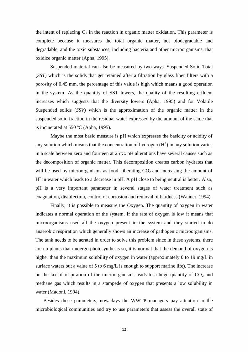
The four classes proposed by Madoni are shown in table 3.
Table 2: SBI Classes (Madoni, 1994)
SBI Value Class Evaluation
8-10 I Stable and well colonized Sludge; optimal biologic
activity; high purifying efficiency
6-7 II Stable and well colonized Sludge; sub-optimal
biologic activity; sufficient purifying efficiency
4-5 III Insufficient biologic activity; mediocre purifying
efficiency
0-3 IV Very low biologic activity; low purifying efficiency
This value, proposed by Madoni in 1994, is based on the specific diversity of the
community as well as its abundance, and in different sensibilities revealed by that
specific population to different physical chemical parameters (Santos, 2008).
There are a lot of advantages of using this method like the use of several
simultaneous criteria such as the numeric and specific richness and the indicator concept
(Santos, 2008).

14
2.7) Organisms Living in WWTP
There is a set of microorganisms living in it like bacteria, yeasts, fungi, algae,
protozoa, metazoa, rotifers, larvae and insects (Oliveira, 1982) and, since this came
from sewage, some of them are pathogenic organisms.
Since protozoa feed by active grazing on bacterial cells, the appear in large
numbers in the system (Madoni, 1994). Some of protozoa are indicators of the good
quality of water treatment (Madoni, 1994). Most protozoa inhabiting the aerating tank
of WWTP are ciliate protozoa. The main function of ciliate protozoa is to be the
predator of the system and they exist in large number (Curds, 1982). Also, flagellate can
be in high numbers. These classes of protozoa possess small number of flagella which
leads to the belief that movement is harder for them then for the previously mentioned
organisms (Seviour and Blackall, 1999).
Fungi are not important members of the common activated sludge process. They
cannot compete with bacteria unless in very low pH (Jenkins et al., 1993).
Referring to metazoan, a large amount of these are nematodes, rotifers and
oligochaete worms, and it is believed that they are bacteria grazers, although, their real
role is not yet truly understood (Ratsak et al., 1993).
In wastewater treatment, bacteria are the dominant group corresponding to 95%
of total microbial population (Martins et al., 2004), in both biomass and number, being
also responsible for the most part of the mineralization and elimination of organic and
inorganic compounds (Amann, 1998, Bitton, 1978).
Bacteria are unicellular prokaryotic organisms and can present different types of
morphology: sphere (cocci) or cylinders (rods or bacilli), rigid blades (vibrios,
spirillum) and flexible helices (spirochetes) (Lopes and Fonseca, 1996). Like all
prokaryotic organisms, there is no nucleolus in the cells and the DNA is located in the
cytoplasm like all the other cell components such as carbohydrates and other organic
complexes that have Ribonucleic acid (RNA) and can synthesize their own proteins, its
dimensions are located between 1 and 3µm in size and 1,5 µm of diameter (Metcalf and
Eddy, 2003). The most common reproductive process is the binary division (Figure 3).
In some cases, the daughter cells stays together which leads to the formation of a
“chain” resulting in the formation of the filamentous forms of bacteria (Nicolau, 2009).

15
Figure 4: bacteria division
Available in <http://science.nayland.school.nz/graemeb/yr11%20work/microbes/bacteria.htm>, acessed in April, 1.
This group includes many fecal commensally bacteria but also pathogenic
bacteria (Grant et al., 1996).
2.7.1) Metabolism of Bacteria
Bacteria are without a doubt very important in chemical changes that occur like
the metabolizing process of the wide diversity of organic compounds present and, in
some advanced plants, bacteria are responsible for the removal of nitrogen and
phosphorus (Seviour and Blackall, 1999); in fact, 91% of all organisms that exist in
activated sludge are bacteria (Nicolau, 2009). In the end, bacteria convert organic and
inorganic nutrients into bacterial cells and inorganic products such as carbon dioxide,
water, ammonia and phosphate (Copper, 2004).
Considering the metabolism of bacteria, they are classified according to the
energy source or the carbon source that they use in the conversion of the substrate
(Nicolau, 2009).
Chemoheterotrophs make up most of the bacteria present in activated sludge
systems. They are aerobic and are responsible for the degradation and utilization of
organic compounds which later turn in cell biomass and CO2 (Painter, 1983).
Chemoautotrophic nitrifying bacteria are the de-nitrificants by excellence
(Robertson and Kuenen, 1992). Nitroso bacteria oxidize NH4+ into NO2
- and Nitro
bacteria oxidize NO2- into NO3
- (Bock et al., 1992). Their growth rates are low and the
energy they release is also low which means that they can be quickly washed out of the
activated sludge system (Painter 1986).
Photoautotrophic and photoheteretrophic bacteria are purple and metabolically
versatile and can denitrify (Hiraoshi et al., 1995).
16
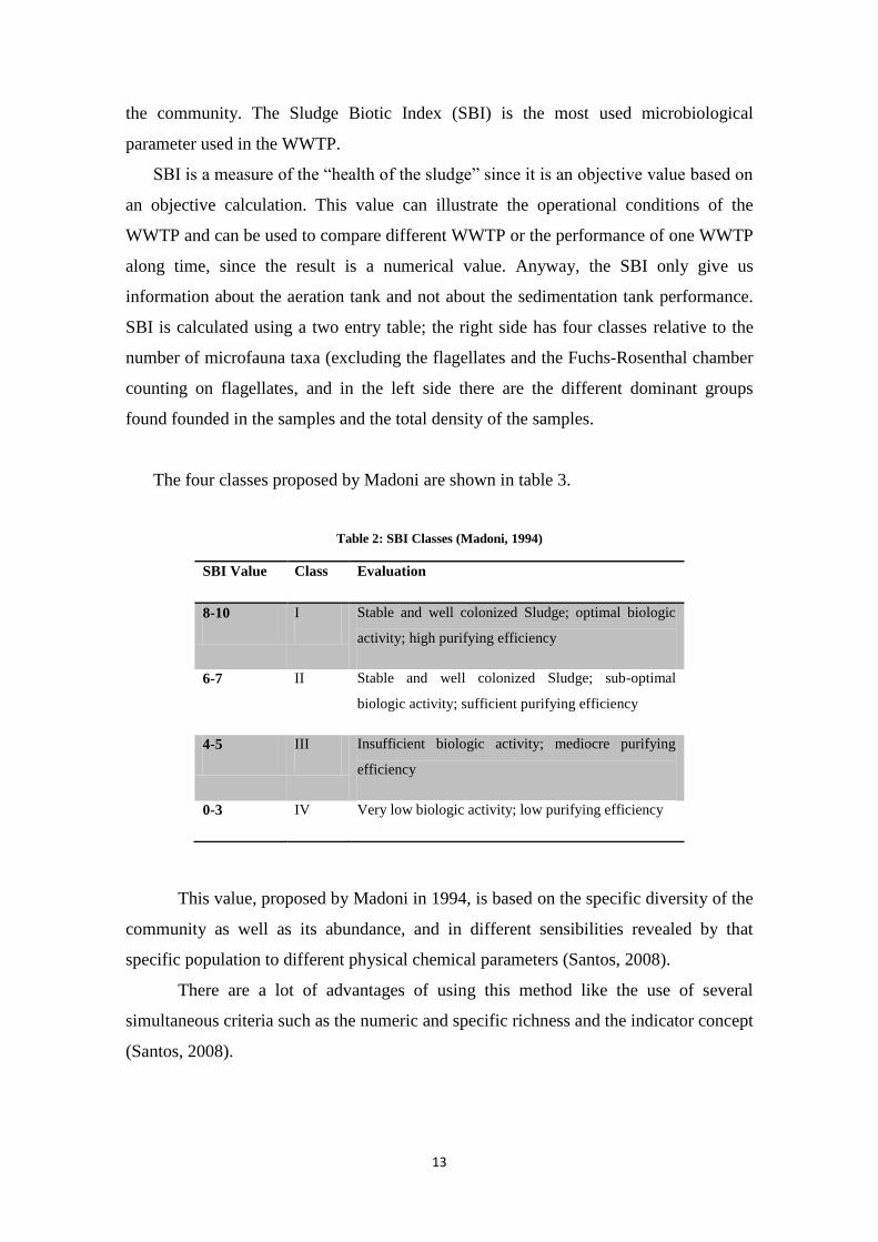
Table 3: Metabolic groups in activated sludge (Nicolau, 2009)
Metabolic Group Carbon Source Energy Source Electron Acceptor Growth Structure
Organotrophs Organic Aerobic Oxidation
FF,FIL
Fermentative
Anaerobes
Organic Fermentation Organic Compound FF
Denitrifiers Organic Anoxic Oxidation
FF,FIL
Nitrifiers Inorganic Aerobic Oxidation
Adhered
Poli-P Organic Aerobic Oxidation
Clusters,FIL
S-oxidizers Inorganic Aerobic Oxidation
FF,FIL
-Reducers Organic Anaerobic Oxidation
FF
In the treatment systems, carbon is the main energy source, so, the dominant
microorganisms are the ones responsible for the metabolism of carbonate compounds.
There are various carbon sources available for organisms, so, its characterization is
measured by the biochemical oxygen demand (BOD) and can be subdivided in
Biodegradable BOD, biochemically modified by the enzymatic system of the organisms
and can be used as a substrate and carbon source, and non biodegradable BOD, either
because it is toxic or the enzymatic system of the organisms cannot degrade them.
These bacteria can be divided in subgroups. They can be organotrophs aerobic and are
bacteria that can remove the most part of the organic compounds in depurating systems
because of its enzymatic system that allows the quick utilization of soluble
biodegradable compounds.
Can be fermentative bacteria and this fermentative process occurs in the absence
of oxygen and nitrates but it is difficult for this process to occur in conventional
systems. These bacteria are responsible for the removal of phosphorus and the
conversion of organic compounds into volatile fatty acids such as acetic acid.
17
Another subgroup is the anoxic bacteria. An example of these is denitrifying
bacteria. These kinds of bacteria have as final electron acceptors nitrates or analogue
substances.
Talking about nitrifying bacteria, these bacteria are responsible for the oxidation
of nitrito to nitrate.
Finally, bacteria can accumulate polyphosphates bacteria: these are of extreme
importance in advanced depuration of residual water, however, their metabolism or
identification is not well understood. It is believed that these bacteria are responsible for
the removal of phosphates (Nicolau; 2009).
2.8.) Advantages of Molecular Methods Vs Classic Methods in the
Identification of Microorganisms
When the research, in the field of wastewater microbiology, first wanted to
identify microorganisms from WWTP, they used very basic methods based on
coloration and microscopic observation. Nowadays, with the advances in molecular
methods, there are a lot of other options available (Gilbride et al., 2006). In order to use
molecular approaches, the very first step is to extract and purify DNA/RNA
(deoxyribonucleic acid/ribonucleic acid) with the nucleic acid it is possible, later, to
obtain pieces of this DNA/RNA belonging to all members of the community regardless
of special growth needs (Talbot et al., 2008). Over the time, molecular approaches have
been very useful and have allowed the identification of new species and has confirmed
older species (Gilbride et al., 2006) and information about the composition, structure,
activity of the microbial community and other kinds of information is always welcome
(Gilbride et al., 2006). Table 4 shows classic and molecular methods of microorganisms
identification. Cultures of microorganism are sometimes done, in order to subsequently
identify them, an appropriate medium is difficult to find. If the aim is to obtain cultures
of all existing microorganisms, the task is increasingly difficult. For example, the
average cell culture count, with the help of a microscope, is 1010
cells/ml (Victoria et
al., 1996) while the number of cells resulting from lab cultures is only 102
or 108
cells/ml (Fulthorpe et al. 1993). In fact, when the number of microorganisms grown in
lab provided from activated sludge is compared with the estimates provided from direct
observation of wastewater prior to cultivation using methods like direct cell counting or
immunochemical techniques, the numbers do not match (Howgrave-Graham and Steyn,
1988).

18
Most of the times, growing cells is time consuming (Kampfer and Dott, 1989)
and can be limited to growing a certain number of bacteria (Amann et al., 2001). Some
molecular methodologies allow cells to be collected right away, cultures grown in labs
show differences in structure and metabolic activity also, one of the most important
advantages is due to molecular approaches the samples can be frozen in order to keep
the metabolic status and microbial composition intact (Widada et al., 2002). Also, with
direct extraction of DNA, information about microorganisms that are not able to grow
in labs but may be responsible for some of the biodegrading activity can be obtained,
which is an important issue (Brockman, 1995). With the use of these techniques it is
possible to understand the diversity and interaction of microorganisms present in the
wastewater.

19
Tab
le 4
: D
iffe
ren
t m
eth
od
s of
mic
roorg
an
ism
id
en
tifi
cati
on
(A
da
pte
d f
ro
m G
ilb
rid
e et
al.
, 2
00
6)
Tec
hn
iqu
e
Ben
efit
s L
imit
ati
on
s E
xa
mp
les
of
usa
ge
Mic
rosc
op
y
Fas
t
Dir
ect
ob
serv
atio
n o
f m
icro
bia
l ce
lls
Maj
ori
ty o
f b
acte
rial
po
pula
tio
n c
anno
t b
e id
enti
fied
A
sso
ciat
ion
of
fila
mento
us
bac
teri
a w
ith
slud
ge
bulk
ing(E
ikel
bo
om
, 1
97
5;
Sei
vo
ur
et a
l.,
19
97)
Med
ia-B
ase
d M
eth
od
s E
asy
to
per
form
Iden
tifi
cati
on
of
ind
ivid
ual
mic
roo
rgan
ism
s
Maj
ori
ty o
f b
acte
ria
canno
t b
e ea
sily
cu
ltiv
ated
on
gen
eral
purp
ose
med
ia
Do
min
atio
n
of
aero
bic
and
fa
cult
ativ
e
anae
rob
ic
het
ero
tro
phs
in kra
ft p
ulp
tr
eatm
ent
syst
em
s (L
iss
and
A
llen,
19
92
)
Co
mm
on b
acte
rial
iso
late
s fr
om
kra
ft b
leac
hed
pulp
mil
l (F
ult
ho
rpe
et a
l.,
19
93
)
Ind
ica
tor
mic
ro
org
an
ism
b
ase
d
pa
tho
gen
est
ima
tio
n
Eas
y
to
per
form
Curr
ent
stand
ard
fo
r co
lifo
rms
Lab
or
inte
nsi
ve
and
ti
me
consu
min
g
Ind
irec
t es
tim
atio
n o
f p
atho
gen
s ra
ther
than d
irec
t
det
ecti
on
Fec
al
coli
form
/fec
al
stre
pto
cocc
us
rati
on
to
dif
fere
nti
ate h
um
an v
s. n
on
-hu
man
po
lluti
on (
Sco
tt
et
al.
,20
02
)
F+
R
NA
and
D
NA
co
lip
hag
e d
ensi
ties
as
an
ind
icat
or
of
wate
r q
ual
ity (
Co
le e
t a
l.,
20
03
)
Am
pli
fied
ri
bo
som
al
DN
A
rest
rict
ion
an
aly
sis
(AR
DR
A)
Cult
ure
-ind
epen
den
t
Suit
able
fo
r an
alysi
s o
f a
wid
e ra
nge
of
mic
roo
rgan
ism
s
DN
A
extr
acti
on
and
P
CR
b
iase
s
No
t q
uan
tita
tive
Mic
rob
ial
div
ersi
ty o
f ac
tivat
ed s
lud
ge (
Bla
ckal
l et
al.
,19
98
; P
elle
gri
n e
t a
l.,
199
9)
Rib
oso
ma
l R
NA
inte
rgen
ic
spa
cer
an
aly
sis
(RIS
A)
Cult
ure
-ind
epen
den
t
Suit
able
fo
r an
alysi
s o
f a
wid
e ra
nge
of
mic
roo
rgan
ism
s
Sig
nif
icant
het
ero
genei
ty
in
length
DN
A
extr
acti
on
and
P
CR
b
iase
s
No
t q
uan
tita
tive
Sig
nif
icant
het
ero
genei
ty
in
len
gth
and
se
quence
Bac
teri
al
div
ersi
ty
and
co
mm
unit
y
analy
sis
fro
m
dif
fere
nt
pu
lp
and
p
aper
w
ast
ew
ater
tr
eatm
ent
syst
em
s (B
aker
et
al.
, 2
003
)

20
and
seq
uence
am
ong b
acte
ria
am
on
g b
acte
ria
Den
atu
rin
g
gra
die
nt
gel
el
ectr
op
ho
resi
s
(DG
GE
)
Cult
ure
-ind
epen
den
t
Suit
able
fo
r an
alysi
s o
f a
wid
e ra
nge
of
mic
roo
rgan
ism
s
Use
o
f rR
NA
gene
seq
uen
ce
het
ero
genei
ty
DN
A
extr
acti
on
and
P
CR
b
iase
s
No
t q
uan
tita
tive
Sp
ecif
icit
y c
an b
e an
iss
ue
bec
ause
of
sho
rt t
arget
seq
uen
ces
Po
pula
tio
n
shif
t (F
erri
s et
a
l.,
19
97
)
Succ
essi
on o
f b
acte
rial
po
pula
tio
n (
Sim
pso
n e
t a
l.,
20
00)
Ter
min
al-
rest
rict
ion
fra
gm
ent
len
gth
po
lym
orp
his
m
(t-
RF
LP
)
Cult
ure
-ind
epen
den
t su
itab
le
for
anal
ysi
s o
f a
wid
e ra
nge
of
mic
roo
rgan
ism
s
Fas
t an
d s
em
i-q
uanti
tati
ve
DN
A e
xtr
acti
on a
nd
PC
R b
iase
s C
om
po
siti
on
of
pulp
m
ill
mic
rob
ial
com
mu
nit
y
(Gil
bri
de
and
Fult
ho
rpe,
20
04)
Bac
teri
al
com
mu
nit
y
com
po
siti
on
fro
m
sew
age
trea
tment
pla
nts
(H
irai
shi
et a
l.,
20
00
)
Flu
ore
scen
t in
si
tu
hy
bri
diz
ati
on
(F
ISH
)
Quanti
tati
ve
Dir
ect
vis
ual
res
olu
tio
n o
f m
icro
bia
l
cell
s in
clu
din
g n
on
-cult
ura
ble
Inac
tive
cell
s m
ay n
ot
be
det
ecte
d
In s
itu
anal
ysi
s o
f m
icro
bia
l co
mm
un
ity s
truct
ure
in
acti
vat
ed
slud
ge
(Wag
ner
et
al.
, 1
99
3)
Ob
serv
atio
n o
f sl
ud
ge
flo
c fo
rmin
g m
icro
org
anis
ms
(Ro
ssel
ló-M
ora
et
al.
,199
5)
Flu
ore
scen
t in
si
tu
hy
bri
diz
ati
on
(F
ISH
)
an
d
con
foca
l sc
an
ing
lase
r
mic
rosc
op
y
Quanti
tati
ve
Dir
ect
vis
ual
res
olu
tio
n o
f m
icro
bia
l
cell
s in
clud
ing
slo
w
gro
win
g
and
no
n-c
ult
ura
ble
Exp
ensi
ve
inst
rum
enta
tio
n
Vis
uali
zati
on o
f nit
rify
ing b
act
eria
(W
agner
et
al.
,
19
98
; Ju
rets
chko
et
al,
. 1
99
8)

21
(C
SL
M)
Mu
ltip
lex P
CR
R
apid
and
sim
ult
aneo
us
det
ect
ion o
f
sever
al t
arget
mic
roo
rganis
ms
Co
mb
inat
ion
s o
f p
rim
er
pai
rs
mu
st
funct
ion
in
a
sin
gle
PC
R r
eact
ion
Det
ecti
on
of
bac
teri
al
pat
ho
gen
s in
w
aste
wate
r
(Ib
ekw
e et
al,
. 2
00
2)
and
vir
use
s (B
eure
t, 2
00
4)
Nu
clei
c a
cid
mic
roa
rra
ys
Hig
h
thro
ug
hp
ut
des
ign
Var
ious
app
lica
tio
ns
Lo
w
sen
siti
vit
y
for
envir
on
men
tal
sam
ple
s
Sam
ple
pro
cess
ing c
om
ple
xit
ies
Pat
ho
gen
det
ecti
on i
n w
ate
r (S
trau
b a
nd
Chan
dle
r,
20
03),
F
ood
s (C
all
et
al.
, 20
01
) an
d
wast
ew
ater
(Lee
et
al.
, in
pre
ss)
On
-ch
ip t
ech
no
log
y
Co
mb
inat
ion
of
PC
R
wit
h
nucl
eic
acid
h
yb
rid
izat
ion
on
a si
ng
le
chip
Les
s in
terf
eren
ce
bet
wee
n
par
alle
l
reac
tio
ns
Inte
gra
tio
n a
nd
pac
kagin
g
Det
ecti
on
of
bac
teri
al
pat
ho
gen
s (L
agal
ly
et
al.
,
20
04
; B
lask
ovic
and
Bar
ak,
20
05
)
22
If classic microbiology is combined with molecular methods, the information
will lead to a more comprehensive perspective and a better interpretation of the in situ
microbial community and its response to engineered bioremediation is possible
(Brockman, 1995).
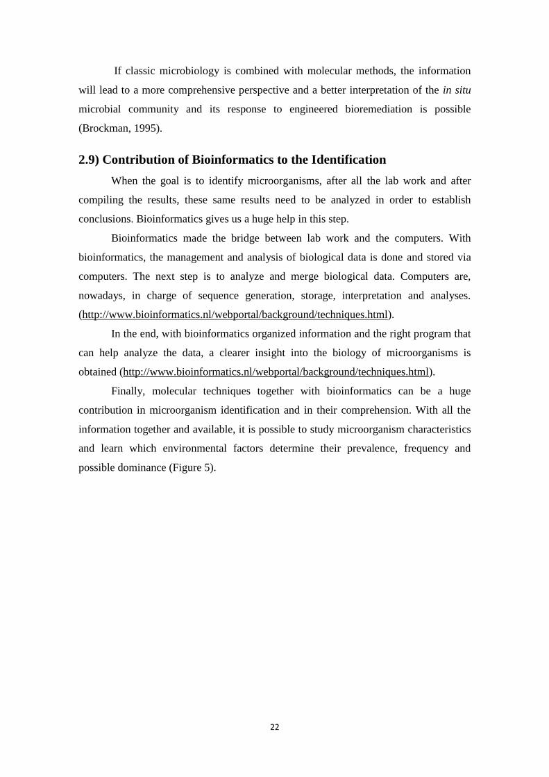
2.9) Contribution of Bioinformatics to the Identification
When the goal is to identify microorganisms, after all the lab work and after
compiling the results, these same results need to be analyzed in order to establish
conclusions. Bioinformatics gives us a huge help in this step.
Bioinformatics made the bridge between lab work and the computers. With
bioinformatics, the management and analysis of biological data is done and stored via
computers. The next step is to analyze and merge biological data. Computers are,
nowadays, in charge of sequence generation, storage, interpretation and analyses.
(http://www.bioinformatics.nl/webportal/background/techniques.html).
In the end, with bioinformatics organized information and the right program that
can help analyze the data, a clearer insight into the biology of microorganisms is
obtained (http://www.bioinformatics.nl/webportal/background/techniques.html).
Finally, molecular techniques together with bioinformatics can be a huge
contribution in microorganism identification and in their comprehension. With all the
information together and available, it is possible to study microorganism characteristics
and learn which environmental factors determine their prevalence, frequency and
possible dominance (Figure 5).

23
Figure 5: Molecular approaches for detection and identification of xenobiotic-degrading bacteria and their
catabolic genes from environmental samples (Adapted from Muyzer and Smalla, 1998)

24
CHAPTER III
Methodology


25
In order to achieve the goal of the present work, a methodology was thought and
applied step by step starting by the sampling of the biological material passing through
the extraction of the DNA and finally the assemblage of the dendrogram.
3.1) Samples
In order to study the microbial biodiversity of the activated sludge process of six
WWTP (Wastewater Treatment Plant), samples were taken from the aeration tank in the
period between and subsequent, then the plating was made in order to obtain a series of
isolates of each sample. A first set of samples, from 2 WWTP, was used to get
acquainted with the methodology: these were samples 2.2MON, 3.2MON, 2.2VZI,
3.2VZI. Next, 4 more WWTP were chosen to complete the study and these latter were
chosen with one year of interval between the two samples of each of the WWTP.
Samples are named as:
2.2.MON
3.2.MON
2.2.VZI
3.2.VZI
2.2.CUC
3.3.CUC
2.2.LAG
3.3.LAG
2.2.SEI
3.3.SEI
2.2.ZIA
3.3.ZIA
3.1.1) Culture of Samples and Isolation of Morphotypes
The samples were cultivated in Tryptone Soy Agar (TSA) (Liofil Chen,
Bacteriology products, Roseto DA, Italy) (Constitution on the appendix II). This
medium was used according to the specifications of the manufacturer and it was chosen
because it possesses a large spectrum of grown organisms. The microorganisms were
plated directly from the samples to a TSA petri dish and grown at 37ºC over 24 hours.
The cultures were observed and the different colonies were tagged and later subculture
to a new Petri dish for another 24 hours in the same conditions. The colonies to
subsequent isolation were chosen among isolated colonies and based on the apparent
differences of colony morphotype. The procedure was repeated as many times as
necessary until the culture appeared to be isolated.
26
3.2) Isolates Preservation
The next step was storing the isolates. In order to do that, the cells were places
from the petri dish directly into a TSB (Tryptic Soy Broth) (Liofil Chen, Bacteriology
products, Roseto DA, Italy) medium (constitution in the appendix II).
The growth was performed during 24 hours to 37ºC with constant agitation and
then 1 ml was taken and centrifuged (Centurion Scientific Ltd) 5 min at 10000 rpm. The
supernatant was rejected. This procedure was performed continuously until a reasonable
quantity of cells was reached.
In order to preserve bacteria, these pellets were suspended in 1ml of TSB (Liofil
Chen, Bacteriology products, Roseto DA, Italy) with 15% of glycerol. In the end, these
preparations were frozen at -80ºC and -20ºC in duplicate.
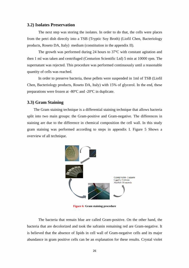
3.3) Gram Staining
The Gram staining technique is a differential staining technique that allows bacteria
split into two main groups: the Gram-positive and Gram-negative. The differences in
staining are due to the difference in chemical composition the cell wall. In this study
gram staining was performed according to steps in appendix I. Figure 5 Shows a
overview of all technique.
Figure 6: Gram staining procedure
The bacteria that remain blue are called Gram-positive. On the other hand, the
bacteria that are decolorized and took the safranin remaining red are Gram-negative. It
is believed that the absence of lipids in cell wall of Gram-negative cells and its major
abundance in gram positive cells can be an explanation for these results. Crystal violet

27
is positively charged. When enters in cells, binds to negatively charged compounds.
With mordant the process is exactly the opposite (James and Mittwer, no year).
Sometimes it is not so easy to say if a bacteria is Gram-negative or Gram-positive
because some organisms have no consistence in results. These organisms are called
gram variable. The results were observed under a microscope (Olympus, CX 41), both
Gram staining results and new fresh preparation, and the results were compared (see
results) using a 100X amplification.
When an isolate had one more morphology than it was assumed that it was not
properly isolated and all the procedure to get an isolate was carried on again.
3.4) Molecular Approaches
The frozen cells were unfrozen and later cultivated again such as in step 2.1.1
conditions in order to move on to a molecular approach. This step was repeated for
every isolate.
3.5) DNA Extraction
In order to obtain DNA to perform PCR the cell lyses were performed. The cells
were directly removed with a loop from the petri dish to 400 µl of a aqueous solution.
The aqueous solution used was made with one solution consisting of 200 µl of 0,5%
SDS, sterilized with a filter (with 0,2µl), plus 200µl of TE buffer (composition in the
appendix II) and were heated at 65ºC for 20 minutes (protocol adapted from Laboratory
for Environmental Pathogens Research, Department of Environmental Sciences
University of Toledo DNA, no year).
3.6) PCR
PCR-fingerprinting is a generic term applied to PCR-based methodologies that
originate a fingerprint of each microorganism. There is a variety of PCR fingerprinting
methodologies; nonetheless, some are based on amplification of different regions of the
genome by PCR, using only one primer. In this work, M13 primer (Invitrogen) was
used. Without question, the major advantage of the PCR-based typing is the fact that the
technique requires very few starting materials, so this makes the technique cheap, has a
universal application and it is rapid to perform (Diaz-Guerra et al., 1997). PCR DNA-

28
fingerprinting consists in applying, ideally, just one specific primer to create a
fingerprint that will be unique to each organism. In order to achieve that goal, it is
important to have low restringing conditions and direct the primer to repetitive
sequences of the genome.
M13 primer has the required conditions. It belongs to the core of M13 phage
mini-satellite that is able, due to low restringing conditions and due to its high affinity
to genome, to amplify several regions of the genome. In fact, this methodology is
employed to amplify hyper-variable genomic DNA sequences (Vassart G. et al., 1987).
M13 primer has the sequence 5’‐GAGGGTGGCGGTTCT‐3’ (Neto, 2008).
The PCR reaction occurred with the help of the high-fidelity enzyme Taq DNA
Polimerase (Invitrogen). The PCR mixtures were done according to the description
below.
Table 5: Composition of DNA mix
Compounds Initial
concentration
Final
concentration
Quantity
Taq 5U 1,25U 0,25 µl
Buffer 10X 1X 2,5 µl
Mg 3mM 1,5mM 1,5 µl
dNTP´s 10mM 4mM 0,5 µl
Primer 50pmol 0,5µM 1,25 µl
DNA
template
X 1:10 dilution 1 µl
Water X X 18 µl
All the reagents used belong to Invitrogen.
The following PCR program was used:
Table 6: PCR program
Steps Conditions Nº of Cycles
Step 1:
Initial Denaturation
3min, 95ºC
1
Step 2:
Denaturation
Annealing
Extention
1min, 95ºC
2min, 50ºC
2min, 72ºC
40
Step 3:
Final Extension
5min, 72ºC
1
4ºC ∞
The reaction mix was made for 25 µl each tube plus one for user errors.

29
DNA was diluted in a proportion of 1:10 (9µl of water plus 1µl of DNA from
damaged cells. This step was performed with intuit of have the perfect amount of DNA
in DNA electrophoresis.
3.7) Electrophoresis Gel
Electrophoresis gel was performed with 1,5% agarose (BioRon) gel prepared
with 1X TAE (Tris-acetate-EDTA) buffer (constitution in appendix II) and PCR
samples were run over 90 minutes at 180 Volts.
Several run times and others buffers were experimented but these were the
conditions that showed the best resolution and the best migration of the pattern band.
The conditions were maintained for all the isolates in order to obtain a platform where it
is possible to compare the results.
Before the polymerization of the agarose (BioRon) 10 mg/ml of ethidium
bromide was added in order to observe the results under UV light.
Table 7: Quantities of ladder and sample for the electrophoresis gel
Ladder 5 µl NZYDNA
Ladder III
Sample 10 µl sample 2 µl loading
TAE buffer is useful in the separation of nucleic acids such as DNA and RNA
and was used in the container before the agarose was there and then was added again
until it covered the gel. The ladder used belongs to NZYTech, Lda and is ready to use.
This molecular weight marker produces a pattern of 14 bands ranging from 200 to
10000 base pair (see appendix III).
3.8) Bioinformatics
To perform the analysis of the isolates obtained, Bionumerics (Applied Maths)
software was the chosen tool. This type of analysis allows the establishment of
correlations between the microbiology, the physical-chemical prevailing parameters
and the performance of the WWTP.
Bionumerics (Applied Maths) software is the only program that can integrate
several techniques like 1D electrophoresis gels, all kinds of spectrometric profiles, 2D
protein gels, phenotype characters, microarrays and sequences in the same platform and
better, this program is able to combine information from various genomic and

30
phenotypic sources in one global database and lead to a conclusive analysis
(http://www.biosystematica.com/bionumerics.pdf). Cluster analysis, is, with no
question, an indispensible tool in bioinformatics, the connections and the flexibility of
relational database with the contribution of multiple techniques (http://www.applied-
maths.com/bionumerics/modules/bn_tn.htm). It is possible to detect and analyze
mutations, make epidemiological typing of bacteria, fungal and virus, bacterial source
tracking, plant and animal breeding and generate the phylogenetic inference and
evolution (Bryan et al., 2004).
The typification of the isolates was done with a M13 primer. This technique was
applied in the analysis of the 113 isolates. After the DNA extraction and amplification
by PCR the M13-PCR fingerprinting profiles were revealed by electrophoresis. Each
profile consists of a complex pattern of bands that categorize each microorganism and
that can be used to differentiate the isolates. The primer used determines the loci
amplified and consequently defines a particular genome sample.
In silico analysis of the densitometry profiles that corresponds to the fingerprints
obtained allowed the construction of the dendrograms applying a coefficient of
correlation “Dice” and a clustering method based on Unweight Pair Group method with
Arithmetic Mean (UPGMA), an optimization of 0,5%, a band Matching Tolerance of
0,5% and a branch quality with cophenetic correlation. The purpose in the analysis of
the dendrograms obtained after the in silico treatment of the M13-PCR fingerprinting
profiles were to group the isolates by cluster similarity.
31
CHAPTER IV
Results and Discussion

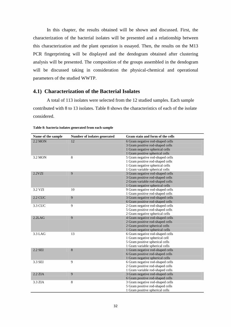
32
In this chapter, the results obtained will be shown and discussed. First, the
characterization of the bacterial isolates will be presented and a relationship between
this characterization and the plant operation is essayed. Then, the results on the M13
PCR fingerprinting will be displayed and the dendogram obtained after clustering
analysis will be presented. The composition of the groups assembled in the dendogram
will be discussed taking in consideration the physical-chemical and operational
parameters of the studied WWTP.
4.1) Characterization of the Bacterial Isolates
A total of 113 isolates were selected from the 12 studied samples. Each sample
contributed with 8 to 13 isolates. Table 8 shows the characteristics of each of the isolate
considered.
Table 8: bacteria isolates generated from each sample
Name of the sample Number of isolates generated Gram stain and form of the cells
2.2 MON 12 6 Gram negative rod-shaped cells
3 Gram positive rod-shaped cells
1 Gram negative spherical cells
1 Gram positive spherical cells
3.2 MON 8 5 Gram negative rod-shaped cells
1 Gram positive rod-shaped cells
1 Gram negative spherical cells
1 Gram variable spherical cells
2.2VZI 9 3 Gram negative rod-shaped cells
3 Gram positive rod-shaped cells
2 Gram variable rod-shaped cells
1 Gram negative spherical cells
3.2 VZI 10 9 Gram negative rod-shaped cells
1 Gram positive rod-shaped cells
2.2 CUC 9 3 Gram negative rod-shaped cells
6 Gram positive rod-shaped cells
3.3 CUC 9 2 Gram negative rod-shaped cells
5 Gram positive rod-shaped cells
2 Gram negative spherical cells
2.2LAG 9 4 Gram negative rod-shaped cells
2 Gram positive rod-shaped cells
2 Gram positive spherical cells
1 Gram negative spherical cells
3.3 LAG 13 6 Gram negative rod-shaped cells
1 Gram negative spherical cell
5 Gram positive spherical cells
1 Gram variable spherical cells
2.2 SEI 8 1 Gram negative rod-shaped cells
6 Gram positive rod-shaped cells
1 Gram negative spherical cells
3.3 SEI 9 6 Gram negative rod-shaped cells
2 Gram positive rod-shaped cells
1 Gram variable rod-shaped cells
2.2 ZIA 9 3 Gram negative rod-shaped cells
6 Gram positive rod-shaped cells
3.3 ZIA 8 3 Gram negative rod-shaped cells
5 Gram positive rod-shaped cells
1 Gram positive spherical cells

33
It is possible to see than Gram negative as well as rod-shaped cells are
predominant in the set of samples: 52,2% of the isolates are Gram negative, 43,4% are
Gram positive and 4,4% are Gram variable; 83,2% are rod-shaped and 16,8% are
spherical. In fact, Gram negative bacteria dominate quantitatively the WWTP
microbiota, but this is not visible in these analyses because the isolates were not
selected to represent the distribution of colonies in the plates. That is, a sample can be
dominated by a gram positive morphotype and only one isolate is selected: the
distribution of bacterial isolates reflects the plating only qualitatively. Gram negative
have a thin cell wall, although they have one second lipid layer which confers an extra
protection to these bacteria making them more resistant to adversities (Prescott et al.,
2009). That can be the reason why gram negative are in higher number than gram
positive that only have one cell wall made of peptidoglycan. In fact, Carvalho and
Fernandes, in 2010, demonstrated that in the sea, Gram negative bacteria respond well
to stressful conditions such as high salinity conditions. The aerated tank of WWTP is
also a much stressed ecosystem and this can be one of the reasons of this slight
dominance.
Gram negative appears when there are a lot of inorganic compounds like
sulfates, nitrites, methane or CO2 (Madoni, 1994).
Out of all the WWTP, the one that has the highest nitrogen load is 3.3ZIA with a
nitrogen load of 209 mg/l, other high values belong to 2.2MON (175 mg/l), 3.3MON
(160mg/l) and 3.2VZI (146mg/l) WWTP.
3.2MON, 2.2LAG, 3.3SEI and 2.2MON, have the highest values of BOD which
means there is a lot of organic matter available to feed microorganism, these WWTP
possesses a majority of gram negative. The COD of these samples are higher than the
BOD because in WWTP not only is biodegradable matter oxidized but non
biodegradable matter is also oxidized (Sawyer, 2003). BOD diminishes in VZI, CUC,
LAG and ZIA WWTP, these systems improved from one year to another.
According to Madonni (1994), the SBI values of the samples 2.2MON, 2.2VZI,
3.2VZI, 2.2CUC, 3.3CUC, 2.2LAG, 3.3LAG, and 2.2ZIA belong to the class I which
means that these systems are very well colonized. Belonging to the class II there are
3.2MON, 3.3SEI and 3.3ZIA. Class II is also a very sufficient system. Belonging to the
class III, there is only 2.2SEI. Besides the low SBI value, WWTP 2.2SEI, as well as
3.3SEI, has a bigger amount of organisms of Opercularia sp. that is one genus that is
particularly resistant to stressful situations such as the presence of certain toxins (such

34
as salts and heavy metals), acidity and lack of oxygen which is the case. This species is
associated with huge amounts of NH4+ that results from catabolism. Looking at the N
concentration on exit, the N has a huge concentration (Seviour and Blackall, 1999). But,
from one year to another (2.2SEI to 3.3SEI), the SBI increased which lead to a
conclusion that the system improved from one year to another.
4.2) Genomic characterization by M13-PCR fingerprinting
With the images obtained after the M13-PCR and subsequent electrophoresis, a
dendrogram was built. It is expected to determine the relationship among samples
considering the clusters obtained. After that, the relationships of the assembled groups
with the characteristics of each of the WWTP are discussed.
The following figure shows an example of a gel with M13-PCR fingerprinting
profiles obtained with Chemi Doc, Biorad, California, for some of the strains in study:
Figure 7: Agarose gel with M13-PCR fingerprinting profiles obtained for some of the strains in study
(Samples: 1-Ladder, 2-Negative control, 3-3.3CUC2.1, 4-3.3CUC3.1, 5-3.3CUC4.1, 6-3.3CUC5.1, 7-3.3CUC7.1, 8-
3.3CUC7.2, 9-3.3CUC8.1, 10-2.2LAG1.2, 11-2.2LAG2.2, 12-2.2LAG4.1, 13-2.2LAG6.1, 14-2.2LAG8.2, 15-
2.2LAG8.1, 16-3.3LAG1.1, 17-3.3LAG2.1, 18-3.3LAG3.1.
Figure 8 shows the dendogram obtained after clustering analysis by the
Bionumerics (Applied Maths) software. The following table (Table 9) shows the
composition of all the groups defined in the dendrogram.
1 2 3 4 5 6 7 8 9 10 11 12 13 14 15 16 17 18 19 20

35

36
Figure 8. Dendogram obtained after clustering analysis.

37
Table 9: Numbers given to the groups of isolates present in dendrogram
Group Isolates
I 2.2VZI4.1, 3.2VZI1.1, 2.2MON4.1, 3.2 VZI6.1, 2.2MON5.2, 2.2MON4.3, 2.2MON5.1
II 2.2MON1.1, 2.2SEI6.1, 2.2CUC1.1, 2.2SEI7.1
III 2.2SEI8.1, 3.3SEI7.1, 3.3SEI6.1
IV 2.2ZIA6.1, 3.2VZI5.2
V 2.2ZIA3.1, 2.2ZIA 4.2, 2.2ZIA4.1, 2.2ZIA1.1, 2.2MON4.2, 3.3SEI8.2, 2.2MON5.1, 3.3CUC1.1
VI 2.2VZI1.1, 3.3SEI8.1, 2.2SEI3.1, 2.2ZIA2.1, 3.3SEI1.1
VII 2.2LAG1.2, 2.2ZIA8.1, 3.3CUC8.1, 3.3LAG6.1, 3.3LAG7.1, 3.2VZI3.1, 3.3CUC4.1, 3.3CUC3.1
VIII 2.2CUC3.1, 3.3LAG3.4, 2.2LAG7.1, 2.2VZI2.1
IX 2.2ZIA7.1, 3.3CUC5.1, 2.2MON1.2, 3.3ZIA3.2, 2.2CUC8.1, 3.3SEI3.2, 3.3SEI3.1
X 3.3ZIA3.1, 3.3ZIA5.1, 3.3LAG2.1, 3.3ZIA5.3, 3.3LAG1.1, 3.3ZIA1.1, 2.2LAG6.1, 3.3ZIA5.2
XI 2.2SEI1.2, 3.3SEI2.1, 2.2CUC1.2, 3.3LAG3.3, 3.3LAG4.1, 3.3LAG3.5, 3.3LAG5.1, 3.3LAG4.2,
3.3LAG5.2
XII a
b
c
2.2MON4.4, 3.2VZI5.3, 3.3LAG3.1, 2.2LAG2.2, 2.2LAG4.1, 3.3ZIA7.1
2.2CUC7.1, 2.2VZI5.1, 2.2MON3.1, 2.2SEI1.1, 3.2MON3.1, 3.3CUC6.1
3.2MON1.1, 3.3CUC7.1, 2.2SEI1.3, 3.3LAG3.2, 3.3ZIA2.1, 3.2MON2.1
XIII d
e
2.2LAG1.1, 3.3CUC2.1, 2.2CUC2.1, 2.2SEI2.1, 2.2MON2.1, 2.2VZI5.2, 2.2VZI5.3
2.2VZI3.1, 3.2MON5.1, 2.2LAG8.1, 2.2LAG8.2
XIV 2.2VZI1.2, 2.2VZI4.2, 2.2VZI4.1
XV 3.2MON1.2, 3.3CUC7.2, 3.2VZI3.2
XVI 3.2MON3.2, 3.2MON3.3, 2.2CUC6.1, 2.2MON3.2
XVII 2.2LAG3.1, 3.2MON2.2, 3.2VZI2.1
Analyzing the dendrogram obtained with the M13-PCR fingerprinting profiles
(Fig.8), it is possible to define seventeen main groups of isolates. In groups XII and
XIII, due to their dimension, subgroups were defined in order to simplify the subsequent
analysis.
The lowest level of similarity was obtained in the group XVII (with about 10%
similarity) and higher level of similarity was among the isolates 3.3LAG3.3 and
3.3LAG4.1 belonging to group XI and 2.2LAG8.1 and 2.2LAG8.2 belonging to group
XIII, specifically in the group XIIIe.

38
The number of isolates in each cluster defined by this technique varied between
two in group IV and eighteen in group XII. In some cases, despite the low level of
similarity (which sometimes is only 25%) is enough to group the bacteria in the same
cluster. The clusters vary in size but all isolates are, in one way or another, related with
the isolates that belong to the same group. In the dendrogram, clusters can be
distinguished from one another and each cluster shares one or several characteristics
with the ones that are related to them. In one first observation it is possible to observe
that the similarity among the isolates is very low, emphasizing the low level of
similarity (21%). In the dendrogram it is possible to verify a significant heterogeneity in
the set of isolates which makes it difficult to create the relation between the groups and
with the characteristics of the WWTP.
Some groups, due to the characteristics of its results, will be presented and
discussed by numerical order.
Group I
The cluster that belongs to group I is composed by seven isolates but these seven
isolates belong to two WWTP: 2.2MON, 2.2VZI and 3.2VZI, although in one WWTP
the samples belongs to different years. The most related isolates belong to different
WWTP. The isolates 2.2MON4.1 and 3.2VZI6.1 share a similarity of 62%. These
isolates (2.2MON4.1 and 3.2VZI6.1) are more closely related with one another than to
the other isolates belonging to the same group and the same WWTP. These samples
share characteristics such as: the range of SSV (228 mg/l in 2.2MON and 292 mg/l in
3.2VZI) and nitrogen that is loaded in the system (175 mg/l in 2.2MON and 146 mg/l in
3.2VZI) and occurrences, although with very different numbers, of Arcella sp. (techaete
amoeba) (2.2MON has 360 ind/ml and3.2VZI has 20 ind/ml), of the crawler ciliate
Acinera uncinata (2.2MON has 2080 ind/ml and 3.2VZI has 60 ind/ml) and of two
attached ciliates: Epistylis sp. (5260 ind/ml in 2.2MON and 4320 ind/ml in 3.2VZI
ind/ml) and Vorticella microstoma (60 ind/ml in 2.2MON and 680 ind/ml in 3.2VZI).
Taking into consideration the Gram staining results, it is possible to see that both
WWTP mostly contain Gram negative rod-shaped cells. More importantly, both WWTP
have an SBI value belonging to a class I category. Maybe all these similarities were
enough allow for the growth of bacteria with a certain similarity.

39
Group V
Another big group formed is the group V. In this group there are 8 isolates. Half
of these isolates belong to the same WWTP, 2.2ZIA. The isolates 2.2ZIA3.1 and
2.2ZIA4.2 are the most related of the group where the similarity percentage between
them is about 62%. In this group of 8 isolates, the four isolates obtained from the
sample 2.2ZIA are the ones that share a higher similarity in the group (2.2ZIA4.1 shares
57% of similarity with the first two and 2.2ZIA1.1 that shares about 42% similarity with
the previous three). The other four isolates, two of them belong to sample 2.2MON.
Nonetheless, the isolate 2.2MON4.2 is more related to 3.3SEI8.2 isolate than to the
other isolate from the same WWTP. These isolates share a similarity of approximately
50%, the same similarity shared by 2.2MON5.1 and 3.3CUC1.1 isolates. All the isolates
are related, in one way or another. This is possible since three of the four WWTP
present in this cluster have an SBI value that belongs to a category of class I. Only the
sample 3.3SEI has a lower SBI which belongs to a category of class II. The sample of
the WWTP 3.3SEI belongs to category of class II and it is more related to WWTP
sample 2.2MON. Both share the same flagellates genera, like Peranena sp. (3.3SEI has
80 ind/ml and 2.2MON also has 80 ind/ml) and the same kind of ciliate crawlers
Acineria uncinata (3.3SEI has 4940 ind/ml and 2.2MON has 2080 ind/ml), the same
attached ciliates Epistylis sp. (3.3SEI has 1800 ind/ml and 2.2MON has 5260 ind/ml)
but 2.2MON has about three times more than 3.3SEI. BOD values are also similar
between 2.2MON, 3.3SEI and 3.3CUC (400 mg/l for 2.2MON, 422 mg/l for 3.3SEI and
341 mg/l for 3.3CUC), COD values (890 mg/l for 2.2MON, 1028 mg/l for 3.3SEI and
1005 mg/l for 3.3CUC), pH values (7,46 for 2.2MON, 7,12 for 3.3SEI and 6,88 for
3.3CUC).
Related to 2.2ZIA WWTP samples, it has an SST loaded similar to 3.3SEI and 2.2MON
WWTP samples (382 mg/l for 2.2ZIA, 428 mg/l for 3.3SEI and 305 mg/l for 2.2MON)
and SSV (330 mg/l for 2.2ZIA, 382 mg/l for 3.3SEI and 228 mg/l for 2.2MON) and
nitrogen load similar to sample 3.3CUC (49.8 mg/l in 2.2ZIA and 53 mg/l in 3.3CUC).
All the WWTP except 3.3CUC have the same flagellates genera, Peranema sp., in
number and specie (80 ind/ml in 2.2MON; 80 ind/ml in 3.3SEI and 60 ind/ml in
2.2ZIA).
The Gram staining showed that in 3.3SEI and 2.2MON there are predominantly
gram negative rod-shaped cells (Table 8) and in 2.2ZIA and 3.3CUC positive rod-
shaped cells prevail. The same conditions along with some shared microorganisms can

40
lead to this similarity. If one WWTP shares microorganisms with another, the isolation
of samples can hook the same microorganisms. One reason for these microorganisms
not being exactly the same can be because in different WWTP the conditions are not the
same. Liu et al., (2001), took several samples during the same day and verified that
depending of the time of the day when the samples were collected, the isolates where
not the same. Certain populations that were present in freshly collected sludge decrease
in abundance over time and can no longer be detected. If this happened during only one
day, in the space of one year, this can also be true. Conversely, other populations are
initially minor members of the community and cannot be detected in freshly collected
activated sludge, but increase in number to become dominant members of the
community after a while (Liu et al., 2001). Maybe the time of collection is grouping the
bacteria form different WWTP in the same group or depend of other such as
reproduction that not always is clonal (Prescott, 2002). That way, if there is sexual
reproduction with plasmids, phages or even transposons, the individuals will be not the
same.
Group VII
Group VII also has eight isolates but shows a greater diversity in terms of
WWTP. The two isolates that show a higher similarity belong to the same WWTP,
3.3LAG (3.3LAG 6.1 and 3.3LAG7.1 sharing 54% similarity. With a slightly lower
similarity there is 2.2LAG1.2 and 2.2ZIA8.1 sharing 50% similarity; these two WWTP
have several characteristics in common such as pH (7.07 in 2.2LAG and 6.88 in
2.2ZIA), the flagellates genera Peranema sp., (80 ind/ml in 2.2LAG and 60 ind/ml in
2.2ZIA), techaete amoeba genera, Arcella sp., (20 ind/ml in 2.2LAG and 740 ind/ml in
2.2ZIA), crawlers ciliate specie, Aspidisca cicada, (100 ind/ml in 2.2LAG and 6020
ind/ml in 2.2ZIA), attached ciliate, Epistylis sp., (5160 ind/ml in 2.2LAG and 1800
ind/ml in 2.2ZIA) and carnivore, Acineta sp., (20 ind/ml in 2.2LAG and 40 ind/ml in
2.2ZIA) although in different quantities. As referred before, these characteristics can be
enough to favor some bacteria over another. These two isolates share a higher level of
intimacy but, are only separated from isolate 3.3CUC8.1 with a similarity of
approximately 43%. The sample 3.3CUC has characteristics in common that make it
possible to put these samples in the same group, such as pH (7,41 in 3.3CUC), nitrogen
load 2.2ZIA (53 mg/l in 3.3CUC and 49.8 mg/l in 2.2ZIA), COD that is similar to
2.2LAG (1562 mg/l in 3.3CUC and 1435 mg/l in 2.2LAG) and the three WWTP have

41
the same crawlers ciliates, Aspicidisca cicada, (940 ind/ml in 3.3CUC). These similar
characteristics may be conducive to the development of similar microorganisms.
3.3VZI3.1 and 3.3CUC4.1 isolates are more closely related than 3.3CUC3.1 and
3.3CUC4.1 isolates, although the three are related. It is important to point out that the
SBI of all the samples in this group belong to a category class I.
Group IX
Group IX has one less isolate in the same cluster than the clusters previously
mentioned. Beyond these seven isolates the ones that are more related, with 61% of
similarity, are the isolates 2.2ZIA7.1 and 3.3CUC5.1. These two isolates were obtained
from a WWTP belonging to an SBI category class I. With about 54% of similarity from
these isolates is 2.2MON1.2. These isolates can be related because the SBI of this
WWTP also belongs to a category class I and the SST load value is similar between the
WWTP samples 2.2MON and 2.2ZIA (305 mg/l in 2.2MON and 382 mg/l in 2.2ZIA).
Looking at the microbiology, 2.2MON and 2.2ZIA have flagellates genera in common,
Peranema sp., (80 ind/ml in 2.2MON and 60 ind/ml in 2.2ZIA), techaete amoeba,
Arcella sp., (360 ind/ml in 2.2MON and 740 ind/ml in 2.2ZIA) and Euglypha sp., (460
ind/ml in 2.2MON and 260 ind/ml in 2.2ZIA), attached ciliate Epistylis sp., (5260
ind/ml in 2.2MON and 220 ind/ml in 2.2ZIA).
In the same sub-group but with low similarity (about 38%), there is 3.3ZIA3.2
isolate. The WWTP 3.3ZIA has an SBI value that belongs to a class II category.
Although the low similarity of clustering, there is some similarities what concerns with
the operational parameters. This isolate shares similar pH with the samples 2.2MON,
2.2ZIA and 3.3CUC (7.54 in 3.3ZIA, 7.46 in 2.2MON, 6.88 in 2.2ZIA and 7.41 in
3.3CUC), SSV; 2.2MON (177 mg/l in 3.3ZIA and 228 mg/l in 2.2MON), COD; 2.2ZIA
(989 mg/l in 3.3ZIA and 1005 mg/l in 2.2ZIA), nitrogen load; 2.2MON (209mg/l in
3.3ZIA and 175 mg/l in 2.2MON mg/L). The gram staining results showed that, in a
general way, this set of samples presents a mix between gram negative and positive rod-
shaped cells as well as some gram variable, but in all the cases, rod-shaped cells prevail.
The isolates 2.2CUC8.1 and 3.3SEI3.2 have a similarity of 54%. They are
distant from the isolate 3.3SEI3.1. These isolates have a similar SST (427 mg/l in
2.2CUC and 428 mg/l in 3.3SEI) and SSV (340 mg/l in 2.2CUC and 382 mg/l in
3.3SEI). Although, they belong to different SBI classes; 3.3SEI belongs to a class II
category and 2.2CUC belongs to a class I category. In the Gram staining results it is
42
possible to see that the rod-shaped cells are mainly gram positive in 2.2CUC and 3.3SEI
has mainly negative rod-shaped cells.
Group X
In group X the isolates 3.3ZIA3.1 and 3.3ZIA5.1 are related with one another
with a 71% similarity and the isolate 3.3LAG2.1 is related with these two with 68%
similarity, having then a fourth isolate, 3.3ZIA5.3, that is related with these three with a
level of similarity of approximately 59%. In this group, samples that come from
WWTP 3.3ZIA are “interrupted” by isolates from 3.3LAG. 3.3ZIA and 3.3LAG can be
related since they show a similar pH (7.54 in 3.3ZIA and 7.13 in 3.3LAG) and a SST
(177 mg/l in 3.3ZIA and 224 mg/l in 3.3LAG). To what concerns to microfauna, there is
crawler’s ciliate Acineria uncinata, (20 ind/ml in 3.3ZIA and 320 ind/ml in 3.3LAG)
and a attached ciliate Epistylis sp. (4260 ind/ml in 3.3ZIA and 80 ind/ml in 3.3LAG).
The next two samples also belong to 3.3LAG and 3.3ZIA and the isolates are related
between themselves with 62% of similarity and these last two are related with the
previous isolates with a similarity of 53%. The next two isolates are related with the
isolates presented before with a percentage of 44% but these two are more similar
between each other, sharing a similarity of 56%, and belong to the WWTP 3.3ZIA and
2.2LAG samples. The curious thing is that between these two WWTP there is not much
in common. Gram staining results between these WWTP shows a prevalence of
negative rod-shaped cells. Contrarily to Wagner et al., 2002, that in geographical areas,
found a better relation between the organisms.
Group XI
The group XI relates two isolates that belong to the same WWTP (SEI) in
different years. This WWTP as modified and that can be seen by the change in SBI
value that changes from five to seven which means a rise from class III to class II. The
similarity is not too high, it is about 53%, but this is enough to group these isolates that
changed a lot in the same cluster. Liu et al. in 2001 verified that in the same WWTP in
different days, not years, the changes in terms of microorganisms were significant. The
result was surprising because sludge from the same wastewater treatment plant were
operated under identical conditions.
Those changes can be possible because the waste continues to come from the
same sources. There is another isolate closely related to these two samples, 2.2CUC7.1.

43
What this sample has in common with the other two isolates is the SST load value
which is similar to 3.3SEI (427 mg/l in 2.2CUC and 428 mg/l in 3.3SEI). In a
microbiological level this last isolate has flagellates protozoa in common with 2.2SEI
and 3.3SEI , Peranema sp., (40 ind/ml in 2.2CUC, 40 ind/ml in 2.2SEI and 80 ind/ml in
3.3SEI), one species of techaete amoeba in common with 3.3SEI, Centropyxis sp., (240
ind/ml in 2.2CUC and 20 ind/ml in 3.3SEI), two crawlers ciliate species in common
with 3.3SEI , Aspidisca cicada, (380 ind/ml in 2.2CUC and 60 ind/ml in 3.3SEI), and
Acineria uncinata (20 ind/ml in 2.2CUC and 4940 ind/ml in 3.3SEI) and share attached
ciliates with 3.3SEI ,Epistylis sp., (40 ind/ml in 2.2CUC and 1800 ind/ml in 3.3SEI).
This can be enough to group these isolates. The next isolates form new group which
includes 3.3LAG. These isolates, as shown in this work, have a tendency of staying
together. In this group it is possible to see one of the two most related samples
3.3LAG3.3 and 3.3LAG4.1, which belong to the same WWTP and to the same year,
and have a similarity percentage of about 90%. With the exception of 2.2CUC, which
Gram staining results showed mostly Gram negative rod-shaped cells.
Group XII
The biggest group that can be found in this dendogram is the group XII. Because
the cluster is so big and it was decided to divide this cluster into three smaller clusters
named XIIa, XIIb and XIIc.
The cluster XIIa includes 6 isolates. The first two isolates belong to different
WWTP and show a 57% similarity. These two isolates 2.2MON4.4 and 3.2VZI5.3, join
with the isolate 3.3LAG3.1 with 32% of similarity possesses an SBI value that belongs
to a category class I which indicates a good level of operation and provides similar
conditions between the WWTP (Santos, 2008). Maybe the reason why different WWTP
are grouped so often next to each other is because of this very fact. The next isolates
belong to the 2.2LAG WWTP (2.2LAG2.2 and 2.2LAG4.1 are related between each
other with 50% of similarity) and, in a smaller level of similarity, these are related with
3.3ZIA7.1 (45% of similarity). This relation already occurred above and the explanation
is the same (see group X). Although the relation between 3.3ZIA and 2.2LAG is
already known, its relation with the rest of the subgroup XIIa is as follows: The pH and
nitrogen entrance of 3.3ZIA (7,54 for pH and 209 mg/l for nitrogen) is similar to
2.2MON (7,46 for pH and 175 mg/l for nitrogen). The BOD of 3.3ZIA (261 mg/l) is
similar with 3.3LAG (225mg/l) and 3.2VZI (240mg/l). 3.3ZIA shares one type of

44
species of techaete amoeba (Arcella sp.) which it has 20 ind/ml, 3.2VZI has 20 ind/ml
and 2.2MON has 360 ind/ml, and shares one species of crawler ciliate (Acineria
uncinata) with 3.3LAG, 3.2VZI and 2.2MON. In 3.3ZIA the quantity is 20 ind/ml, in
3.3LAG, 320 ind/ml in 3.2VZI, 60 ind/ml and in 2.2MON 2080 ind/ml. All these
similarities could provide some conditions where some microorganisms survive and for
this reason, they look similar in a molecular point of view (Tabka et al., 1993).
Considering the Gram staining results of the WWTP from which these isolates originate
it is possible to see a higher inclination towards negative rod-shaped cells with some
WWTP showing a balance between negative and positive rod-shaped cells.
In the subgroup XIIb there are two different isolates that share a similarity of
50%, 2.2CUC7.1 and 2.2VZI5.1, this value is not too high. Up until this point, when
similarities are not too high, it is more and more difficult to find similarities in physico-
chemical characteristics but these two samples have an SBI value that belongs to the
category of class I and this stability can be favorable for the development of similar
microorganisms. 2.2MON3.1 is the most related isolate with these two samples (40% of
similarity) and its SBI value is also of a category class I. Related with these isolates
there is 2.2SEI1.1 and 3.2MON3.1 with 35% of similarity with the previous isolates and
46 % with each other. These WWTP are different in many aspects and even their SBI
value (5 class II for 2.2SEI and 7 which means class III for 3.2MON WWTP) is
different. 3.3CUC6.1 is least similar of the group with a similarity of only 25% and it
has an SBI value of 9 meaning it is in a category of class I. The Gram staining results
for this Group demonstrate a preference for positive rod-shaped cells although 2.2VZI
has a balance of negative and positive rod-shaped cells and 2.2CUC, 3.3CUC and
2.2SEI seem to have more positive rod-shaped cells.
In the subgroup XIIc, 3.2MON1.1 and 3.3CUC7.1 are related with 2.2SEI1.3.
The SBI class of this last one is of a category class III while 3.2MON belongs to a class
II category and 3.3CUC belongs to a class I category. All these WWTP belong to a
different SBI class. The similarity percentage is not too high (53% between 3.2MON1.1
and 3.3CUC7.1 and 37% between these two and 2.2SEI1.3). This percentage is low but,
even so, these samples are in the same group. Sometimes, in genetic terms,
microorganisms that are different are related in small way since all organisms,
following the evolutionary trail, are related. When organisms are found with a low
similarity between them, this can be the reason. The other three isolates are less related
with the previous three and these are 3.3LAG3.3, 3.3ZIA2.1 that are related between

45
each other with 50% of similarity and share 41% of similarity with 3.3MON2.1. Only
the 3.3LAG isolate has a WWTP that has an SBI belonging to a category of class I.
These three samples share with the previous three samples a similarity of only 24%. The
Gram staining results for this group do not vary much from the other XII groups
showing a higher affection for negative rod-shaped cells with one example (2.2SEI) of
mostly positive rod-shaped cells and two examples (3.3CUC and 3.3LAG) of a balance
between positive and negative rod-shaped cells.
Group XIII
The group XIII was also divided into two subgroups (XIIId and XIIIe). In XIIId
the isolates 2.2LAG1.1 and 3.3CUC2.1 belong to different WWTP but they share a 40%
similarity. Related to these two isolates there are another two slightly better related,
sharing a 42% similarity. These isolates are 2.2CUC2.1 and 2.2SEI2.1. These last pair
isolates share a 30% similarity with the first pair. Truth is, at this stage, similarities are
rare. Related with these four isolates is 2.2MON2.1 with a similarity close to 22%. This
is a very heterogeneous group. All these isolates, except from 2.2SEI, have an SBI
value that belongs to a category of class I. Related to these isolates, with 20% of
similarity are the isolates 2.2VZI5.2 and 2.2VZI5.3 that show a 100% similarity with
one another. Taking into consideration how the samples were isolated and these two
came from the same Petri dish it is possible that they are indeed the same organism.
Visually the band pattern is very similar.
In XIIIe the isolates 2.2LAG8.1 and 2.2LAG8.2 share 90% of similarity because
they came from the same WWTP and are related with a 43% similarity to the isolates
2.2VZI3.2 and 3.2MON5.1 which share a similarity with one another of 50%. The
Gram staining results for this group XIII (XIIId and XIIIe) show a balance between
positive and negative rod-shaped cells having two WWTP with a higher affection for
negatives, two with a higher affection for positives and two with a balance between both
negative and positive rod-shaped cells.
Initially, it was expected that the samples would group according to their
geographical localization like in the study of Liu et al. (2001) that in its results indicate
that the microbial community structure of activated sludge varies between
geographically distinct wastewater treatment plants. In this study a pattern like this was
not verified. When someone studies patterns of species, they get the idea that it is easy
to establish a correlation between species and how certain species relate to each other.

46
But when a set of samples originate from a heterogeneous group, an obvious
relationship is not expected in the assemblage (Sugihara et al., 2003). In this work the
heterogeneity originates from geographical parameters as well as from different seasons
and years of the sample collection was verified. In work of Liu et al., 2001, they
assumed that all the disparity between the groupings is attributed, despite the reasons
due to differences in wastewater composition and plant operation that affect the
structure of the indigenous microbial communities. In this case, the reason cannot be
this one because the same WWTP are separated from the isolates that belong to the
same WWTP. Residuals can change with geographical location but also depend on the
level of life of the people that inhabit certain areas; once again, the geographical region
of these samples is almost the same which exclude this hypothesis. Also, Portugal is
such a small country and microorganisms have a tendency to be similar. In this study
this was not verified because, despite of the similarity level, the similarity was not very
high in any isolate.
Tabka et al., (1993) and Liu et al., (2001), found that activated sludge from
different wastewater treatment plants does vary from one wastewater treatment plant to
other but the reason why the microorganisms are so different between the same WWTP
remains unknown.
Liu et al, 2001 and Wagner (1993) assumed that WWTP in different continents
clustering together suggesting that there is a microbial community in geographical
regions. The isolates in my results are mixed together. It would be interesting take
another geographical region and do the same treatment with the goal of see if that
isolates form two different populations based on the geographical regions
Different clusters can yield different dendrograms in aspect (Legendre and
Legendre, 1983) and for single linkage methods like this one whose only parameter is a
genetic parameter (Sugihara et al., 2003) advocate UPGMA as the best method.


47
CHAPTER V
Conclusions and Future Work


48
Upon finishing the present work some conclusions can be achieved. Being a
exploratory work, similar work to relate with the present results was difficult to find,
making the discussion even harder.
Beside the fact that the microorganisms grouped, they grouped with low
similarity. Even when isolates grouped with a higher similarity, the similarity was never
really that high. Even in Gram staining results, all samples showed Gram negative and
Gram positive isolates with no indication of a pattern.
The isolates did not show any pattern in their distribution. Even the Geographical
regions did not group together frequently.
In conclusion, molecular techniques together with bioinformatics can have a
significant contribution to the study and comprehension of the complex communities of
activated-sludge systems, namely the prokaryotic component.
In the future, the same analyses can be made with different primers in order to
confirm and see better the relations between the microorganisms. Also, different
molecular techniques can be used. As an example it is possible enumerate; random
amplification of polymorphic DNA (RAPD), restriction fragment length polymorphism
(RFLP) detection and southern hybridizations with various repetitive sequence-based
probes. Techniques like these are able to group microorganisms and assure that the
isolates are in the right group. In recent years, methods that couple PCR and rRNA
based microbial phylogeny have been developed and used to assess the diversity within
microbial communities in terms of the kinds and relative abundance of various
phylogenetic groups of organisms.
Some authors thought in better ideas that can be applied in the future. While the
data obtained cannot be directly translated into taxonomic terms (i.e., species), the
concept of an operational taxonomic unit (OTU) can be employed to provide a way to
overcome this problem (Moyer et al., 1996). Instead of comparing communities based
on the analysis of cloned 16S rDNA, the OTU richness and evenness (of numerically
dominant members of the community) are estimated from restriction site
polymorphisms or differences in the melting behavior of the 16S rDNA genes. Both of
these methods provide insight to the diversity of 16S rDNA genes (or OTUs) present in
a community, while obviating the need for extensive sequence analysis. However
measures of microbial diversity based on differences in 16S rDNA genes are also
limited because, while they provide an estimate of the number and kinds of

49
phylogenetically distinct groups of organisms in the community, they do not provide
direct measures of genetic diversity per se.
Another interesting approach, just with the intention of seeing how Portuguese
microorganisms behave, another geographical region could be chosen and its results
compared with the results from this work in order to try and find a pattern in Portuguese
population.

50
CHAPTER VI
Bibliography


51
Amann, R., Fuchs, B.M. and Behrens, S. (2001). The identification of microorganisms by fluorescence
in situ hybridization. Current Opinion in Biotechnology, 12:231–236.
Amann, R., Lemmer, H. and Wagner, M. (1998). Monitoring the community structure of wastewater
treatment plants: a comparison of old and new techniques. FEMS Microbiology Ecology. 25, 205-
215.
Apha (1995). Standard methods for the examination of water and wastewater. 19th edn American
public health association, Washington DC.
Betancourt, W.Q. and Rose, J.B. (2004). Drinking water treatment processes for removal of
Cryptosporidium and Giardia. Vet. Parasitol., 126(1–2), 219–234.
Bitton, G. (1978). Survival of enteric viruses. In Water Pollution Microbiology ,Vol. 2 (ed. R.
Mitchell), pp. 273–300, Wiley Interscience, New York, USA
Bock, J. K., Loebell, H. and Morey, R. (1992). From conceptual roles to structural relations: Bridging
the syntactic cleft. Psychological Review, 99, 150-171.
Bonde, G.J. (1977). Bacterial indication of water pollution. In Advances in AquaticMicrobiology (eds. M.R.
Droop and H.W. Jannasch), pp. 273–364. AcademicPress, London.
Bott, C.B. and Love, N.G. (2002). Investigating a mechanistic cause for activated sludge
deflocculation in response to shock loads of toxic electrophilic chemicals. Water Environmental
Research, 74 (3), 306-315.
Brockman, F.J. (1995). Nucleic acid based methods for monitoring the performance of in situ
bioremediation. Mol. Ecol. 4: 567-578.
Bryan, A., Shapir, N. and Sadowsky, M.J. (2004). Frequency and distribution of tetracycline
resistance genes in genetically diverse, nonselected, and nonclinical Escherichia coli strains isolated
from diverse human and animal sources. Appl Environ Microbiol. 70:2503–7.
Carvalho, C.R. and Fernandes, P. (2010). Production of Metabolites as Bacterial Responses to the
Marine Environment. Mar. Drugs. Vol. 8. pp.705-727.
Codd, G.A. (1995). Cyanobacterial toxins: occurrence, properties and biological significance. Wat.
Sci. Tech., 32, 4: 149-156.
52
Cooper, S. (2004). Bacterial Growth and Division. In Encyclopedia of Molecular and Cellular Biology
and Molecular Medicine. Meyers, R.A. (ed), Weinheim, Germany: Wiley-VCH, pp. In Press.
Curds, C.R. (1982). The ecology and role of protozoa in aerobic sewage treatment processes. Annu.
Rev. Microbiol., 36, 27-46.
Diaz-Guerra T.M., Martinez-Suarez J.V., Laguna F. and Rodriguez-Tudela J.L. (1997). Comparison of
four molecular typing methods for evaluating genetic diversity among Candida albicans isolates
from human immunodeficiency viruspositive patients with oral candidiasis. J Clin Microbiol 35:856-
861.
Eckenfelder, W.W. (1978). Technical consideration of biological, physical and chemical treatment
combination for improved efluent quality from industrial wastewater. Prog Water Technol., 10:
434±441.
Flores-Alsina, X., Comas, J., Rodriguez-Roda, I., Gernaey, K.V. and Rosen, C. (2009). Including the
effects of filamentous bulking sludge during the simulation of wastewater treatment plants using a
risk assessment model. Water Research, 43: 4527-4538.
Frey, W. (1992). A comparison of different aeration systems. Water Sci. Technol., 25, 143-149.
Fulthorpe, R.R., Liss, S.N. and Allen, D.G. (1993). Characterization of bacteria isolated from a
bleached Kraft pulp mill wastewater treatment system. Can. J. Microbiol. 39, 13–24.
Gilbride, K.A., Lee, D.Y. and Beaudette, L.A. (2006). Molecular techniques in wastewater:
Understanding microbial communities, detecting pathogens, and real-time process control. Journal
of Microbiological Methods, 66, 1–20.
Grant, S.B., Pendroy, C.P., Mayer, C.L., Bellin, J.K. and Palmer, C.J. (1996). Prevalence of
enterohemorrhagic Eschichia coli in raw and treated municipal sewage. Appl. Environ. Microbiol.,
62, 3466-3469.
Gray, N.F. (1990). Activated Sludge: Theory and Practice. Oxford: Oxford University Press.
Gray, N.F. (1999). Water Technotogy-an Introduction for Scientists and Engineers. Oxford: Boston
Elsevier/Butterworth-Heinemann.
Guide Water UK. (2006).
Hansen S, Mehlum JE and Bakken LR (1993). N20 and CH4 fuxes in soil influenced by fertilization
and tractor traffic. Soil Biol Biochem., 25,621-630.

53
Hawkes, H. A. (1983). Activated Sludge. in Ecological aspects of used-water treatment, 2, Londres,
Academic Press, 1983, pp. 77-162.
Higgins, M.J. and Novak, J.T. (1997). Dewatering and Settling of Activated Sludges: The Case for
Using Cation Analysis. Water Environment Research. Vol. 69, No. 2 (Mar. - Apr., 1997), pp. 225-232.
Hiraoshi, A., Muramatsu, K. and Urato, K. (1995). Characterization of new denitrifying Rhodobacter
strains isolated from photosynthetic sludge to wastewater treatment. J. Ferm. Biogen., 79, 39-44.
Howgrave-Graham, A.R. and Steynm, P.L. (1988). Application of the fluorescent-antibody technique
for the detection of Sphaerotilus natans in activated sludge. Appl Environ Microbiol., 54, 799-802.
Jenkins, D., Ramadori, R. and Cingolani, L. (1993). Prevention and Control of Bulking Activated
Sludge. Centro Luigi Bazzucchi, Perugia.
Jenkins, D., Richard, M.G. and Daigger, G.T. (2004). Manual on the Causes and Control of Activated
Sludge Bulking, Foaming, and Other Solids Separation Problems. London: Lewis Publishers.
Kampfer, P. and Dott, W. (1989). Numerische Identiflzierung aquatischer Mikroorganismen mittels
automatisierter Methoden am Beispiel von Bakterien aus dem belebten Schlamm. Zbl Bakt Hyg. B,
187, 216-229.
Larsdotter, K. (2006). Microalgae for phosphorus removal from wastewater in a Nordic climate. A
Doctoral Thesis from the School of Biotechnology, Royal Institute of Technology, Stockholm, Sweden,
ISBN: 91-7178-288-5.
Lee, N.M. and Welander, T. (1996). Use of protozoa and metazoa for decreasing sludge production in
aerobic wastewater treatment. Biotechnol Lett 18: 429±434
Legendre, P. and Legendre L. (1983). Numerical ecology. Develop. Environ. Model. V. 3. Elsevier.
Lens, P. and Stuetz, R. (2004). Water and Environment Management Series. Alliance House Street,
London UK. 3º Edition.
Liu, W.T., Marsh, T.L., Cheng, H. and Forney, L. J. (1997). Characterization of microbial diversity by
determining terminal restriction fragment length polymorphisms of genes encoding. 16S rRNA. 63,
4516-4522.
Lopes, A. M. and Fonseca, Á. (1996). Biologia Microbiana. Universidade Aberta.

54
Madoni, P. (1994). A sludge biotic index (SBI) for the evaluation of the biological performance of
activated sludge plants based on the microfauna analysis. Water Res., 28:67-75.
Madoni, P., Davoli, D. and Chierici, E. (1993). Comparative analysis of the activated sludge
microfauna in several sewage treatment works. Water Res., 27:1485–91.
Martins, A.M., Pagilla, K., Heijnen, J.J. and Loosdrecht, M. (2004). Filamentous bulking sludge - a
critical review. Water Res., 38:793-817.
Matsui, S., Barrett, F.D. and Banerjee, J. (1991). Guidelines of Lake Management. Toxic Substances
Management in Lakes and Reservoirs. International Lake Environment Committee Foundation, Otsu.
Vol. 4. 170 pp.
Megank, M.T.J. and Faup, G.M. (1988). Enhanced biological phosphorus removal from
WasteWaters. Biotreatment Syst., 3, 111-204.
MetCalf and Eddy, I. (2003). Wastewater engineering: treatment and reuse. 4ª Edition. McGraw-Hill
Higher.
Moyer, C. L., Tiedje, J. M., Dobbs, F. C., and Karl, D. M. (1996). A computer-simulated restriction
fragment length polymorphism analysis of bacterial small-subunit rRNA genes: Efficacy of selected
tetrameric restriction enzymes for studies of microbial diversity in nature. Appl. Environ. Microbiol.
62, 2501-2507.
Muyzer, G. and Smalla K. (1998). Application of denaturing gradient gel electrophoresis (DGGE)
and temperature gradient gel electrophoresis (TGGE). in microbial ecology.
Neto, M. (2008). Alterações na Comunidade Microbiana de um Solo Contaminado com Gasóleo.
Tese de Mestrado, Faculdade de Ciências e Tecnologia, Universidade Nova de Lisboa.
Nicolau, A. (2009). Identificação de problemas ao Nível do Decantador e Controlo do Crescimento
Filamentoso. 1º Nível. Biotempo, Consultoria em Biotecnologia.
Oliveira, J.S. (1982). Operações e processos fundamentais em engenharia sanitária. Fundamentos da
depuração biológica. Faculdade de Ciências e Tecnologia. Universidade Nova de Lisboa.
Painter, H.A. (1978). Biotechnology of wastewater treatment. In the oil industry and microbial
ecosystems. Chater, K. and Someville, H (ed.), London, Heyden and son.
55
Painter, H.A. (1983). Metabolism and physiology of aerobic bacteria and fungi. In Ecological Aspects of
Used Water Treatment, Vol. 2 (eds. C.R. Curds andH.A. Hawkes), pp. 11–75. Academic, London.
Painter, H.A. (1986). Nitrification in the treatment of sewage and wastewater. Nitrification (ed. J.I.
Prosser), IRL Press, Aberdeen, pp. 185-211.
Prescott, L., Harley, J. and Klein, D. (2005). Microbiology. 6th edition McGraw-Hill
Prescott, L. et al,. (2009). Microbiology. 7th
edition Wm. C. Brown Publishers. (Unit – 1, 4)
Ratsak, C.H., Koojiman, S.A.L.M. and Kooi, B.W. (1993). Modelling the growth of an oligochaete on
activated sludge. Water Res. 27, 739-747.
Robertson, L.A. and Kuenen, J.G. (1992). Nitrogen removal from water and waste. Microbial Control
of Pollution. Cambridge University Press, Cambridge, pp. 227-267.
Rocher, M., Goma, G., Pilas Begue, A., Louvel, L. and Rols, J.L. (1999). Towards a reduction in excess
sludge processes: Biomass physicochemical treatment and biodegradation. Addlied Microbiology
Biotechnology, 51, 883-890.
Sahlstrom, L., Aspen, A., Bagge, E., Danielsson-Tham, M.L. and Albihn, A. (2004). Bacterial pathogen
incidences in sludge from Swedish sewage treatment plants. Water Res. 38, 1989–1994.
Santana, F., Amaral, L. and Maurício, R. (2009). Técnicas de Drenagem e Tratamento de Águas
Residuais. Faculdade de Ciências e Tecnologia, Universidade Nova de Lisboa.
Santos, L. (2008). Avaliacao do desempenho de estacoes de tratamento de aguas residuais atraves da
observacao da comunidade de protozoarios nos sistemas de lamas activadas. Tese de Mestrado,
Escola de Engenharia, Universidade do Minho.
Sawyer, C.N. (2003). Chemistry for Environmental Engineering and Science. 5th
Edition. NewYork.
Tata McGraw-Hill
Seviour, R.J. and Blackall, L.L. (1999). The Microbiology of Activated Sludge. Kluwer Academic
Publishers.
Sneath, P. H. A., Mair, N. S., Sharpe, M. E., Holt, J. G. (1986). Bergey's manual of systematic
bacteriology. Vol. 2. Williams and Wilkins Co., Baltimore.

56
Sugihara, G., Bersier, L.F., Southwood, T.R.E., Pimm, S.L. and May, R.M. (2003). Predicted
correspondence between species abundances and dendrograms of niche similarities. PNAS vol. 100
No. 9.
Tabka, H., Seignez, C., Adler, N., Pulgarin, C. and Peringer, P. (1993). Inoculum standardization for
biodegradability tests. Biotechnol. ¹echn. 7, 217-222.
Talbot, G., Topp, E., Palin, M.F. and Masse, D.I. (2008). Evaluation of molecular methods used for
establishing the interactions and functions of microorganisms in anaerobic bioreactors.
Waterresearch. 42, 513 – 537.
Tandoi V., Jenkins D. and Wanner J. (2006). Activated sludge separation problems. IWA Publishing,
London.
Vassart, G., Georges, M., Monsieur, R., Brocas, H., Lequarre, A.S. and Christophe, D. (1987). A
sequence in M13 phage detects hypervariable minisatellites in human and animal DNA. Science,
235, 683-684.
Victoria, L., Gilbride, K.A., Allen, D.G. and Liss, S.N. (1996). Phenotypic fingerprinting of microbial
communities in wastewater treatment systems. Water Res., 30, 1077–1086.
Wagner, M., Brumelis, D. and Gehr, R. (2002). Disinfection of wastewater by hydrogen peroxide or
peracetic acid: Development of procedures for measurement of residual disinfectant and
application to a physicochemically treated municipal effluent. Water Environ. Res., 74: 33-50.
Wanner, J. (1994). Activated sludge population dynamic. Water Sci. Technol. 30, 159-169.
Widada, J., Nojiri, H. and Omori, T. (2002). Recent developments in molecular techniques for
identification and monitoring of xenobiotic-degrading bacteria and their catabolic genes in
bioremediation. Appl Microbiol Biotechnol. 60, 45–59.
Websites:
http://science.nayland.school.nz/graemeb/yr11%20work/microbes/bacteria.htm. Accessed in
December, 2011.
http://weather.nmsu.edu/Teaching_Material/SOIL350/waste_water_treatment_plant.htm. Accessed in
January, 2011.

57
http://www.akvo.org/wiki/index.php/Activated_Sludge. Accessed in December, 2011.
http://www.bioinformatics.nl/webportal/background/techniques.html. Accessed in January , 2011.
http://www.piercenet.com/browse.cfm?fldID=5558F7E4-5056-8A76-4E55-4F3977738B63. Accessed in
December, 2011.
http://www.purdue.edu/rem/hmm/ethidbr.htm. Accessed in February, 2011.
http://www.biosystematica.com/bionumerics.pdf. Accessed in December, 2011.
http://www.applied-maths.com/bionumerics/modules/bn_tn.htm. Accessed in January, 2011.


58
Appendix


59
Appendix I
Gram staining process:
First, a colony was selected and a sterilized loop was used in order to prepare a thin
layer of sample in a glass slide glass.
The previous colony was resuspended in a water drop previously placed in the
slide.
The smear was air dried
Then, the coloration was made:
The smear was placed inside a recipient containing Crystal violet by 1 minute.
The slide glass was cleaned with running water.
The smear was placed inside a recipient containing Lugol’s solution for 1
minute.
The slide glass was cleaned with running water.
30 seconds dropping alcohol drop by drop in to the slide glass
The smear was placed inside a recipient containing safranine solution for 1
minute (see better detailed description in the appendix).
Gram staining consists in the following steps;
Primary stain; (Crystal violet, methyl violet or Gentian violet). The primer dye is
a stable solution and may contain a mordant with the goal of making the
constancy of the solution. Sodium bicarbonate can also be added with the
objective of intensifying the color. Alkaline pH is better (Sheppe and Constable,
1923).
Mordant; Gram’s iodine (James and Mittwer, with no year).
Decolorize; (ethyl alcohol, acetone or 1:1 ethanol-acetone mixture). Most of the
times, the alcohol used is 95%, but acetone can also be used or a mixture of
alcohol and acetone (Lillie, 1928). This is the most critical step in all the process
because there is a danger for both over and under discoloration (Neide, 1904)
Counterstain; (Dilute carbol fuchsin, safranin or neutral red) (James and
Mittwer, no year).
60
Appendix II:
Mediums and buffers composition
TSB
Formula / Liter
Enzymatic Digest of Casein ................................................. 17.0 g
Enzymatic Digest of Soybean Meal ....................................... 3.0 g
Sodium Chloride ................................................................. 5.0 g
Dipotassium Phosphate ........................................................ 2.5 g
Dextrose ............................................................................. 2.5 g
Final pH: 7.3 ± 0.2 at 25°C
TSA
Trypticase peptone..........................................................1.5%
Phytone peptones............................................................0.5%
NaCl...............................................................................0.5 %
Agar.................................................................................1.5%
Enzymatic Digest of Casein and Enzymatic Digest of Soybean Meal are nitrogen
sources in TSB. Dextrose is the carbon energy source that facilitates organism growth.
Sodium Chloride maintains osmotic balance and Dipotassium Phosphate is a buffering
agent. This medium was weighted just like the TSA medium.
TE buffer
For 1 liter of 1x TE solution
1M Tris-HCl pH 7.5 or 8.0…………………10ml/10mM
0.5M EDTA pH 8.0…………………………2ml/1mM
ddH2O………………………………………..998ml

61
TAE
In its composition there is Tris-acetate buffer, usually at pH 8.0, and EDTA, which
sequesters divalent cations (Ogden and Adams, 1987).
Buffer was weighed in an analytic scale in a 1L shot, was agitated with a magnetic
agitator and then was put inside the electrophoresis
10X TBE Electrophoresis Buffer
Tris Base………………………….108g
Boric Acid…………………………55g
0.5M EDTA……………………….20ml
Water to 1.0 L

62
Appendix III
DNA ladder:
Figure 8: Ladder NZYDNA ladder III with corresponding band size

63
A
pp
end
ix I
V
Thes
e ta
ble
s bel
on
g t
o t
he
pro
ject
PR
OT
OF
ILW
WW
W a
nd a
re n
ot
resu
lts
of
my w
ork
, al
thou
gh, th
ese
par
amet
ers
are
esse
nti
als
for
the
rela
tion
bet
wee
n d
iffe
rent
resu
lts:
Tab
le 1
0:
Ph
ysi
co-c
hem
ical
ch
ara
cteri
stic
s
WW
TP
ID
02 m
g/L
(AT
) p
H
SS
T
mg
/L
(AT
)
SS
V
mg
/L
(AT
)
SS
T
(In)
SS
T
(Out)
S
ST
%
SS
V
(In)
SS
V
(Out)
SS
V
%
N m
g/L
(In)
N m
g/L
(Out)
N
tota
l%
BO
D
(In)
BO
D
(Out)
B
OD
%
CO
D
(In)
CO
D
(Out)
C
OD
%
2.2
.MO
N
2,8
6
7,4
6
26
05
19
00
30
5
5
98
22
8
3
99
17
5
18
90
40
0
6
99
89
0
48
95
3.2
.MO
N
1,5
3
7,2
4
38
20
29
60
42
3
12
97
36
3
9
98
16
0
8
95
80
0
14
98
10
80
37
97
2.2
.VZ
I 0
,51
7,5
4
26
80
19
30
15
6
2
99
10
2
1
99
12
10
17
25
7
8
97
35
9
24
93
3.2
.VZ
I 2
.00
-5.0
0
6-9
2
69
0
20
30
45
6
4
99
29
2
3
99
14
6
50
66
24
0
9
96
56
0
61
89
2.2
.CU
C
6,3
5
8,4
3
44
00
28
33
42
7
6
99
34
0
4,4
9
9
77
18
77
20
3
8,7
9
6
81
5
27
97
3.3
.CU
C
0,2
2
7,4
1
46
33
31
32
11
07
8
99
73
7
5
99
53
3,6
9
3
16
1
4
98
15
62
30
98
2.2
.LA
G
1,2
6
7,0
7
56
00
42
00
66
8
4,2
9
9
56
3
2,4
1
00
82
,5
5
94
48
3
8
98
14
35
35
98
3.3
.LA
G
1,1
5
7,1
3
29
33
19
33
26
4
8
97
22
4
5
97
,8
67
,4
15
77
,74
22
5
21
91
50
8
45
91
2.2
.SE
I 0
,45
7,1
8
44
67
33
67
23
6
21
91
19
8
17
91
50
21
,7
57
29
6
8
97
69
9
64
91
3.3
.SE
I 0
,16
7,1
2
34
33
28
34
42
8
23
95
38
2
20
95
92
21
77
42
2
15
96
10
28
53
95
2.2
.ZIA
3
,27
6,8
8
39
22
28
44
38
2
8,8
9
8
33
0
6,8
9
8
49
,8
9,3
3
81
34
1
8
98
10
05
26
,9
97
3.3
.ZIA
0
,14
7,5
4
45
67
37
32
20
7
33
84
17
7
26
85
20
9
19
4
7
26
1
46
82
98
9
59
3
40

64
T
ab
le 1
1:
Mic
rob
iolo
gic
Ch
aracte
rist
ics
(in
d/m
L).
Pro
tozoa (
pa
rt 1
)
Fla
gel
late
s T
echae
te a
mo
eba
Fre
e-sw
imm
ers
WW
TP
ID
Per
an
ema
sp.
Fla
gel
ado
no
t
iden
tifi
ed 1
Arc
ella
sp.
Eu
gly
pha
sp.
Cen
tro
pyx
is
sp.
Co
lpid
ium
sp.
Cin
eto
chil
um
ma
rga
rita
ciu
m
Sp
iro
sto
mu
m
tere
s
2.2
.MO
N
80
3
60
46
0
3.2
.MO
N
2.2
.VZ
I 2
0
2
60
6
0
3.2
.VZ
I
2
0
2.2
.CU
C
40
1
1
78
0
24
0
2
00
3.3
.CU
C
2.2
.LA
G
80
2
0
40
6
0
3.3
.LA
G
40
14
0
2.2
.SE
I 4
0
60
38
0
3.3
.SE
I 8
0
2
0
2.2
.ZIA
6
0
7
40
26
0
40
0
3.3
.ZIA
2
0
4
0

65
T
ab
le 1
2:
Mic
rob
iolo
gic
Ch
aracte
rist
ics
(in
d/m
L).
Pro
tozoa (
pa
rt 2
)
C
raw
lers
cil
iate
s
WW
TP
ID
Ch
ilo
do
nel
la
un
cin
ata
Tri
thig
mo
sto
ma
cucu
llu
lus
Tro
chil
ia
min
uta
Asp
idis
ca
cica
da
Asp
idis
ca
lyn
ceu
s
Eu
plo
tes
pa
tell
a
Oxy
tric
ha
sp.
Aci
ner
ia
un
cin
ata
Aci
ner
ia
incu
rva
ta
Mic
roth
ora
x
sp.
2.2
.MO
N
20
20
80
3.2
.MO
N
78
0
2.2
.VZ
I
15
420
3.2
.VZ
I
72
80
6
0
6
0
2.2
.CU
C
20
38
0
1
20
3.3
.CU
C
40
1
00
94
0
38
0
46
0
2.2
.LA
G
1
00
2
0
3.3
.LA
G
3
20
2.2
.SE
I
3.3
.SE
I 8
0
34
0
6
0
4
94
0
2.2
.ZIA
60
20
3.3
.ZIA
1
20
20
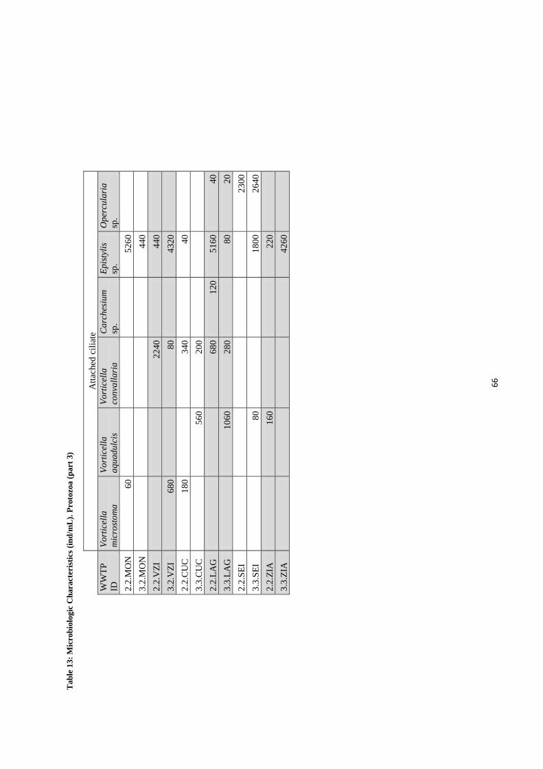
66
T
ab
le 1
3:
Mic
rob
iolo
gic
Ch
aracte
rist
ics
(in
d/m
L).
Pro
tozoa (
pa
rt 3
)
A
ttac
hed
cil
iate
WW
TP
ID
Vo
rtic
ella
mic
rost
om
a
Vo
rtic
ella
aq
uad
ulc
is
Vo
rtic
ella
con
vall
ari
a
Ca
rch
esiu
m
sp.
Ep
isty
lis
sp.
Op
ercu
lari
a
sp.
2.2
.MO
N
60
5
26
0
3.2
.MO
N
44
0
2.2
.VZ
I
2
24
0
4
40
3.2
.VZ
I 6
80
8
0
4
32
0
2.2
.CU
C
18
0
3
40
4
0
3.3
.CU
C
5
60
20
0
2.2
.LA
G
68
0
12
0
51
60
40
3.3
.LA
G
1
06
0
28
0
8
0
20
2.2
.SE
I
23
00
3.3
.SE
I
80
18
00
26
40
2.2
.ZIA
16
0
22
0
3.3
.ZIA
4
26
0

67
T
ab
le 1
4:
Mic
rob
iolo
gic
Ch
aracte
rist
ics
(in
d/m
L)ç
. P
roto
zoa (
part
4)
C
arniv
oro
us
SB
I
WW
TP
ID
Co
lep
s
hir
tus
Lit
on
otu
s
sp.
Aci
net
a
sp.
To
kop
hry
a
sp.
Dis
cop
hry
a
sp.
Pla
gio
cam
pa
rou
xi
Ca
rniv
oro
(n
ot
iden
tifi
ed)
Suct
ori
a (n
ot
iden
ifie
d.
1)
0
2.2
.MO
N
9
3.2
.MO
N
6
0
7
2.2
.VZ
I
20
9
3.2
.VZ
I
9
2.2
.CU
C
40
4
0
40
0
10
3.3
.CU
C
9
2.2
.LA
G
20
9
3.3
.LA
G
9
2.2
.SE
I
2
0
5
3.3
.SE
I
2
20
7
2.2
.ZIA
5
20
4
0
1
24
0
1
10
3.3
.ZIA
7

68
Appendix V
Gram staining results:
2.2CUC
Figure 9: 2.2CUC
(2.2CUC1.1- Negative bacillus. This cells are different from every cells obtained.
Seemed like it have litle ball inside the cells ; 2.2CUC1.2- Gram negative bacillus;
2.2CUC2.1- Gram positive bacillus in a red background; 2.2CUC3.1- Bacillus gram
positive; 2.2CUC4.1- gram positive in a red background. The cells have spors;
2.2CUC5.1- Bacillus positive with spors; 2.2CUC6.1- Gram negative bacillus;
2.2CUC7.1- Gram positive bacillus; 2.2CUC8.1-Gram positive bacillus).
3.3CUC
Figure 10: 3.3CUC
(3.3CUC1.1-Gram positive with some negative cells; 3.3CUC2.1- Coccus gram
negative; 3.3CUC3.1- Bacillus gram positive but a few gram negative; 3.3CUC4.1-
Bacillus some gram positive and others gram negative; 3.3CUC5.1-Bacillus gram
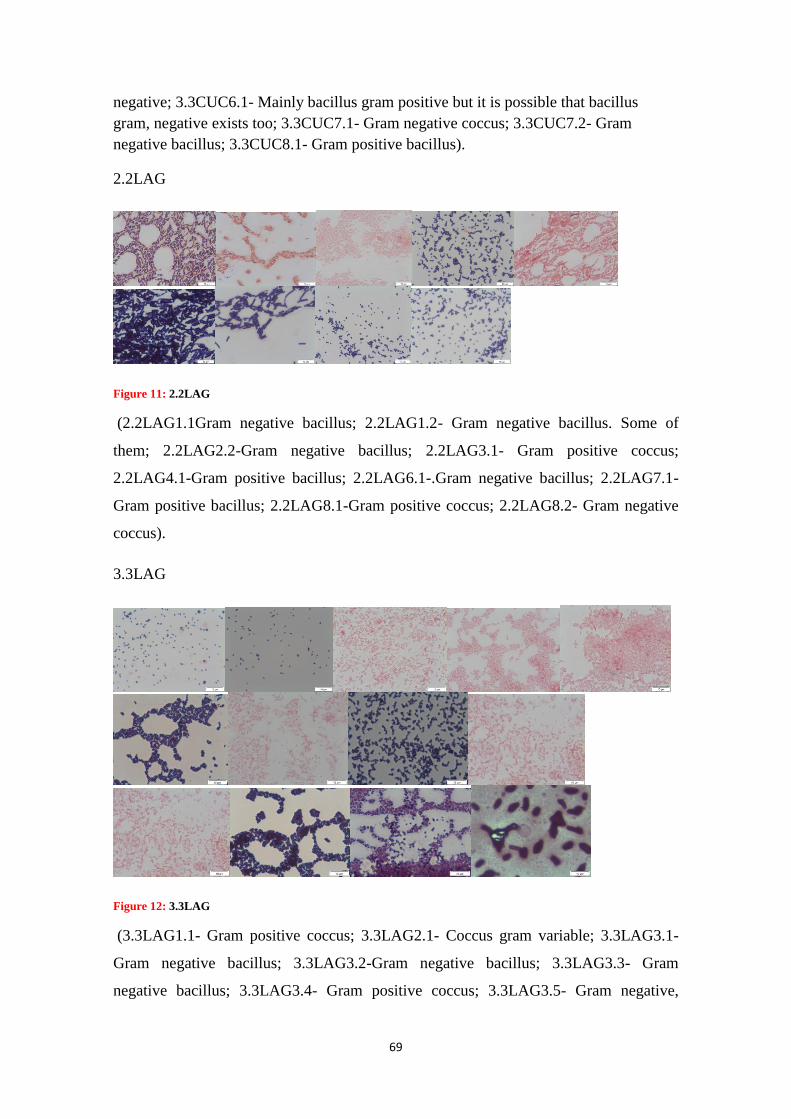
69
negative; 3.3CUC6.1- Mainly bacillus gram positive but it is possible that bacillus
gram, negative exists too; 3.3CUC7.1- Gram negative coccus; 3.3CUC7.2- Gram
negative bacillus; 3.3CUC8.1- Gram positive bacillus).
2.2LAG
Figure 11: 2.2LAG
(2.2LAG1.1Gram negative bacillus; 2.2LAG1.2- Gram negative bacillus. Some of
them; 2.2LAG2.2-Gram negative bacillus; 2.2LAG3.1- Gram positive coccus;
2.2LAG4.1-Gram positive bacillus; 2.2LAG6.1-.Gram negative bacillus; 2.2LAG7.1-
Gram positive bacillus; 2.2LAG8.1-Gram positive coccus; 2.2LAG8.2- Gram negative
coccus).
3.3LAG
Figure 12: 3.3LAG
(3.3LAG1.1- Gram positive coccus; 3.3LAG2.1- Coccus gram variable; 3.3LAG3.1-
Gram negative bacillus; 3.3LAG3.2-Gram negative bacillus; 3.3LAG3.3- Gram
negative bacillus; 3.3LAG3.4- Gram positive coccus; 3.3LAG3.5- Gram negative,

70
coccus; 3.3LAG4.1-Gram positive coccus; 3.3LAG4.2- Gram negative bacillus;
3.3LAG5.1- Gram negative bacillus; 3.3LAG5.2- Gram positive, coccus; 3.3LAG6.1-
Gram positive coccus; 3.3LAG7.1- Gram negative bacillus).
2.2MON
Figure 13: 2.2MON
(2.2MON1.1-Bacillus gram negative; 2.2MON2.1-Bacillus gram negative; 2.2MON3.1-
Gram positive bacillus in a negative background; 2.2MON3.2- Bacillus gram negative;
2.2MON4.1-gram negative in a positive background; 2.2MON4.2-Gram positive
bacillus; 2.2MON4.3-gram positive bacillus in a positive background; 2.2MON4.4-
Coccos gram negative; 2.2MON5.1-gram negative bacillus; 2.2MON6.1-Bacillus gram
negative; 2.2MON6.2-positive coccus).
3.2MON
Figure 14: 3.2MON
(3.2MON1.1- Bacillus gram negative; 3.2MON1.2- Gram negative, Bacillus;
3.2MON2.1- Gram negative bacillus; 3.2MON2.2- Mainly gram negative bacillus but

71
there is some positive cells; 3.2MON3.1- Negative and positive Coccus; 3.2MON3.2-
Gram negative bacillus; 3.2MON3.3- Coccus gram negative; 3.2MON5.1- Gram
positive in a negative background).
2.2SEI
Figure 15: 2.2SEI
(2.2SEI1.1-Bacillus gram positive; 2.2SEI1.2-Cocos gram negative; 2.2SEI1.3-Bacillus
with red background gram positive; 2.2SEI2.1-Bacillus gram positive; 2.2SEI3.1-Big
bacillus ; 2.2SEI6.1-Bacillus with red background gram positive; 2.2SEI7.1-Bacillus
gram negative; 2.2SEI8.1-Bacillus with red background gram positive).
3.3SEI
Figure 16: 3.3SEI

72
(3.3SEI1.1-Bacillus gram negative; 3.3SEI2.1-Bacillus gram negative; 3.3-SEI3.1-
Bacillus gram negative; 3.3SEI3.2-Bacillus gram negative; 3.3SEI5.1-Bacillus gram
negative; 3.3SEI6.1-Bacillus gram variable; 3.3SEI7.1-Bacillus gram negative;
3.3SEI8.1-Bacillus gram positive and coccos gram negative; 3.3SEI8.2-Bacillus with
red background gram positive).
2.2VZI
Figure 17: 2.2VZI
(2.2VZI1.1-Bacillus with red background gram positive; 2.2VZI1.2-Bacillus gram
variable; 2.2VZI2.1-Bacillus gram negative; 2.2VZI3.1-Bacillus gram negative;
2.2VZI4.1-Bacillus gram positive; 2.2VZI4.2-Bacillus gram variable; 2.2VZI5.1-Cocos
gram negative and Bacillus gram positive; 2.2VZI5.2-Bacillus gram negative;
2.2VZI5.3-Bacillus gram positive).
3.2VZI
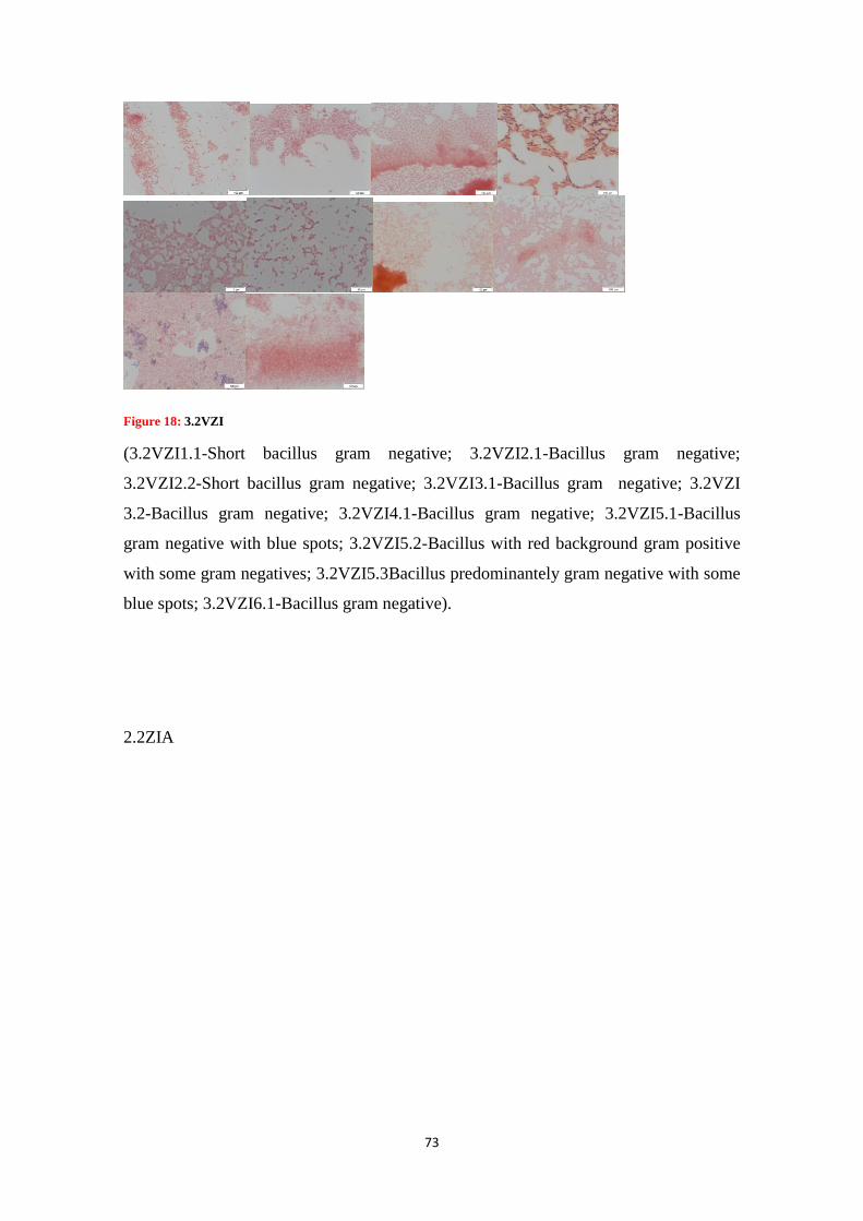
73
Figure 18: 3.2VZI
(3.2VZI1.1-Short bacillus gram negative; 3.2VZI2.1-Bacillus gram negative;
3.2VZI2.2-Short bacillus gram negative; 3.2VZI3.1-Bacillus gram negative; 3.2VZI
3.2-Bacillus gram negative; 3.2VZI4.1-Bacillus gram negative; 3.2VZI5.1-Bacillus
gram negative with blue spots; 3.2VZI5.2-Bacillus with red background gram positive
with some gram negatives; 3.2VZI5.3Bacillus predominantely gram negative with some
blue spots; 3.2VZI6.1-Bacillus gram negative).
2.2ZIA
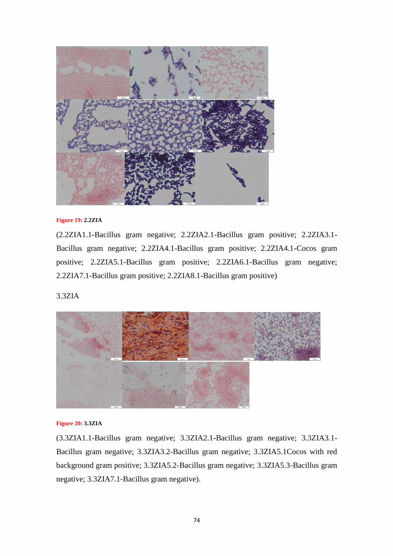
74
Figure 19: 2.2ZIA
(2.2ZIA1.1-Bacillus gram negative; 2.2ZIA2.1-Bacillus gram positive; 2.2ZIA3.1-
Bacillus gram negative; 2.2ZIA4.1-Bacillus gram positive; 2.2ZIA4.1-Cocos gram
positive; 2.2ZIA5.1-Bacillus gram positive; 2.2ZIA6.1-Bacillus gram negative;
2.2ZIA7.1-Bacillus gram positive; 2.2ZIA8.1-Bacillus gram positive)
3.3ZIA
Figure 20: 3.3ZIA
(3.3ZIA1.1-Bacillus gram negative; 3.3ZIA2.1-Bacillus gram negative; 3.3ZIA3.1-
Bacillus gram negative; 3.3ZIA3.2-Bacillus gram negative; 3.3ZIA5.1Cocos with red
background gram positive; 3.3ZIA5.2-Bacillus gram negative; 3.3ZIA5.3-Bacillus gram
negative; 3.3ZIA7.1-Bacillus gram negative).