guía de uso de datos de audiencia - nielsen ibope

GUÍA DE USO DEDATOS DE AUDIENCIA

2

Nielsen IBOPE México

DERECHOS RESERVADOS © NIELSEN IBOPE MÉXICO, S.A. DE C.V.Blvd. Manuel Ávila Camacho 191, piso 5, Col. Polanco I Sección

La presente obra contiene materiales propiedad Industrial e Intelectual de Nielsen IBOPE México S.A de C.V. por lo que se prohíbe su reproducción permanente o temporal, total o parcial, por cualquier medio y de cualquier forma; su traducción, adaptación, reordenación y cualquier otra modificación; su distribución del original o copias de la base de datos; su comunicación al público, y su reproducción, distribución o comunicación pública. La violación estará sancionada como lo disponen las leyes en la materia.

3

Guía para el uso de datos de audiencia

Introducción

Glosario básico

1. Número mínimo de casos para analizar un target

1.1. ¿Cuál es el número mínimo de casos conforme a lineamientos internacio-nales?

1.2. ¿Qué se recomienda hacer cuando hay un número pequeño de casos de un target en la muestra?

2. Consultas de targets con pocos casos en muestra

2.1. ¿Cómo utilizar las variables de análisis en consultas de target con pocos casos en muestra?

2.2. ¿Qué tipo de agregados pueden disminuir la variabilidad del dato?

3. Alcance y Frecuencia durante el periodo de rotación del panel

3.1. ¿Qué variaciones se pueden esperar en los resultados de Alcance y Fre-cuencia durante una campaña publicitaria?

3.2. ¿Qué se recomienda para disminuir la variación en la post-evaluación y la planeación?

Contenido

4. Variable Error Estándar Relativo en la MSS

4.1 Uso e interpretación de la variable Error Estándar Relativo

5. Consideraciones adicionales

5.1 Consideraciones para el análisis de audiencia por Series de Tiempo

4


Gran cantidad de usuarios de la información de audiencias de televisión de Nielsen IBOPE se ha encontrado alguna vez con el dilema de saber y entender cuál es el número mínimo de casos de un target en muestra para realizar con-sultas de ratings con “robustez estadística”.

Sobre el tema existen prácticas y recomendaciones que distintos actores de la industria de medios suelen seguir para la realización de análisis, planeación o estrategias de negociación. Lo cierto es que éstas no siempre se fundamentan en información estadística entendible para ser aplicadas por los profesionales que no son expertos en estadística.

Dado lo anterior, el presente Manual tiene por objetivo ayudar a los usuarios a entender de una forma sencilla y amigable cómo reducir los errores estándar provenientes de la consulta de estimadores de una muestra.

En este documento encontrará recomendaciones específicas sobre el número de casos en muestra para el uso de targets y variables de análisis, así como de Alcance y Frecuencia durante un corto periodo de tiempo de rotación del pa-nel, así como otros factores a considerar en la realización de los análisis de la información.

Estas recomendaciones resultan de gran importancia para el uso e interpreta-ción adecuada de los datos de audiencia de Nielsen IBOPE México, exhortamos a la industria de medios a aplicarlas ya que resultan buenas prácticas a seguir por los tomadores de decisiones.

Introducción

5


Error estándar de un rating: es la diferencia del rating de la muestra respecto al de una población completa.

Margen de error de un rating: es un intervalo en puntos de rating, con límites máximos y mínimos, dentro del cual puede moverse el rating de la muestra respecto al de una población completa, y con base en ello determinar un rango de confianza. El rango más usual se define a 95% de confianza.

Error relativo: es el resultado de dividir el error estándar de un rating entre el valor total del rating. Se utiliza regularmente para comparar el error como porcentaje de distintos valores y tamaños de rating. * Todos estos conceptos estadísticos son aplicables a otras variables de audiencia.

Glosario básico

6


1. Número mínimo de casos para analizar un target

Para que el usuario minimice o contenga el incremento del error estándar durante el proceso de rotación del panel las dos variables más importantes que se deben tener en cuenta son los casos que hay de un target en la muestra y el tamaño del estimador consultado (rating, Alcance, ats, etc.).

1.1. ¿Cuál es el número mínimo de casos conforme a lineamientos internacionales?

Existen lineamientos internacionales que determinan el número mínimo de casos en la muestra que valida el indicador de audiencia (Anexo 1).

Según los estándares del Media Rating Council (MRC) en Estados Unidos, el número mínimo de casos en muestra recomendado para permitir el análisis de un target es de 30 casos. El Global Guidelines for Televi-sion Audience Measurement (GGTAM) tiene lineamientos más conservadores que aplican principalmente en Europa. Nielsen en Estados Unidos se rige por el número mínimo de casos de GGTAM, y en México se aplica lo sugerido por el MRC. En el software de consulta de Nielsen IBOPE se establecen 30 casos en muestra como un nivel mínimo para el cálculo de estimadores.¹

Estos distintos lineamientos se fundamentan estadísticamente en el tamaño de los errores estándar (Anexo 3).

1.2 ¿Qué se recomienda hacer cuando hay un número pequeño de casos de un target en la muestra?

El actual fenómeno de fragmentación de las audiencias de televisión a nivel global, el cual ha generado la disminución del tamaño de los ratings y llevado a las industrias a trabajar con errores estándares relativos más altos, invita a analizar con mayor detalle el número mínimo de casos necesarios de muestra.

Para estimaciones o tamaños pequeños de rating es importante aplicar otras medidas para que el usuario pueda minimizar o contener el error estándar de los datos (ejemplo en Anexo 4).

¹En el módulo de creación de targets en los software Media Quiz y Media Smart Station es posible observar por colores (rojo, amarillo y verde) la identificación del número de casos con el que se trabaja un target en un análisis específico: rojo = 30 casos o menos (no utilizar), amarillo = 31 a 49 casos (utilizar con reservas) y verde más de 50 casos (análisis con mayor estabilidad). Para mayor ilustración ver Anexo 2.

7


2. Consultas de targets con pocos casos en muestra Resulta una práctica común en la industria realizar análisis de audiencias a partir de la definición de targets de consulta perfilados (hábitos de consumo, estilos de vida, etc.), bajo el entendido de que una mayor definición del target conlleva a mayor precisión acerca del grupo objetivo al que se desea llegar, situación sólo cierta si se cuenta con un tamaño de muestra suficiente. Por tanto se debe tener en cuenta que:

Al crear un target de consumo de televisión es poco recomendable utilizar demasiadas va-riables demográficas, ya que entre más demográficos se seleccionen, menor es el número de casos, lo cual genera variabilidad en los datos. La integración de individuos que no son parte del target, pero que tienen características demográfi-cas similares, puede contribuir a dar estabilidad de los resultados sin impactar demasiado al público objetivo. De lo contrario, se tendrán que considerar intervalos de confianza más amplios.

2.1. ¿Cómo utilizar las variables de análisis en consultas de target con pocos casos en muestra?

Establecer la prioridad entre las diferentes variables de análisis ayuda a minimizar o contener el error, pues-to que el error incrementa a medida que se hacen análisis con la mínima expresión de cada variable, así:

Target: (Mínima expresión permisible por el software: 30 casos)Vehículo: (Mínima expresión permisible: 1 canal) Horario: (Mínima expresión permisible: 1 minuto)Periodo: (Mínima expresión permisible: día)

8


Una vez elegida la variable principal del análisis, por ejemplo si fuera un programa, se recomienda robus-tecer el resto:

Target: si se eligen hombres 19+ ABC+ en Guadalajara y este target tiene menos de 200 casos en muestra, es posible robustecerlo agregando mujeres 19+ ABC+ en Guadalajara, dado que el programa en cuestión es de un género para todo público. En el supuesto que el género fuera particular, se podría robustecer con segmentos de edad y/o nivel socioeconómico inmediatos, hasta llegar al punto de integrar otros dominios.Vehículo: si el programa es transmitido en más de un canal, se incluirían estos canales. Periodo: permite consultar la audiencia del programa en un día específico y analizarlo tantas veces como haya sido transmitido.

2.2. ¿Qué tipo de agregados pueden disminuir la variabilidad del dato?

Existen prácticas en distintos mercados que también utilizan estimaciones con muestras que minimizan o con-tienen el error estándar aplicando promedios. Por ejemplo, Nielsen realizó un análisis considerando ratings pun-tuales por minuto respecto a ratings con otro tipo de agregados. Dicho análisis llegó a la siguiente conclusión:

Este análisis logra reducir el error estándar al realizar distintos promedios respecto el rating específico de un minuto.

El error estándar de un rating promedio de varios minutos (por ejemplo, el de un programa) será menor que el error estándar de un rating del mismo

tamaño que provenga de un minuto en específico.

9


3. Alcance y Frecuencia durante el periodo de rotación del panel

3.1. ¿Qué variaciones se pueden esperar en los resultados de Alcance y Frecuencia durante una campaña publicitaria?

La rotación de un panel completo en un corto periodo de tiempo puede llegar a generar una mayor varia-bilidad en los datos de audiencia en comparación a la que regularmente se observa en un panel estable.Las variabilidades detectadas en las estimaciones de audiencia diaria no muestran incremento significativo conforme a un plan de rotación correctamente implementado; sin embargo, las estimaciones de variables del panel constante como Alcance y la Frecuencia pueden reflejar mayor afectación debido al cambio rá-pido de los hogares en la muestra a lo largo del tiempo. Dado lo anterior:

La rotación genera una baja de Alcance respecto al que una misma campaña suele lograr con base en un panel estable.Los GRP no resultan impactados en forma significativa, por ende la Frecuencia tiende a subir de manera sostenida a raíz de la baja de Alcance.Es importante que el usuario considere los siguientes promedios de baja de Alcance y alza de Frecuencia como una magnitud de los movimientos observados y no como tasa de ajuste puntual, ya que en los distintos targets analizados² se registraron diferencias con mayor o menor importancia.- La baja de Alcance suele ser mayor a medida que las campañas se sostienen durante más tiempo, como ejemplo los siguientes datos:

-1.5% de Alcance promedio en campañas mensuales-6.4% de Alcance promedio en campañas trimestrales-14.7% de Alcance promedio en campañas semestrales

- El incremento de Frecuencia suele ser mayor a medida que las campañas se sostienen por más tiempo, como ejemplo los siguientes datos:

+1.6% de Frecuencia promedio en campañas mensuales+6.8% de Frecuencia promedio en campañas trimestrales+17.3% de Frecuencia promedio en campañas semestrales

Ver Anexo 5.

²Total personas con guest, personas 19+ con guests, personas 19+ sin DE con guest, personas 4-12 con guests, amas de casa, mujeres ABC+C 19-44 con guest, mujeres CD+ 19-44 con guest, hombres ABC+C 19-44 con guest, hombres CD+ 19-44 con guest, personas ABC+C 19-44 con guest, personas CD+ 19-44 con guest, amas de casa ABC+C, amas de casa CD+, personas 4-12 ABC+C con guest, personas 4-12 CD+ con guest, personas 13-18 ABC+C con guest, personas 13-18 CD+ con guest, total

hogares.

10


3.2. ¿Qué se recomienda para disminuir la variación en la post-evaluación y la planeación?

Las siguientes recomendaciones, tanto para la planeación como para la post-evaluación, son producto de todas aquellas señaladas en esta guía, y otras que surgen a partir de sugerencias hechas en otros mercados como el inglés, con base en un análisis presentado en el congreso internacional de ESOMAR, Broadcast Audience Research, en Viena, Austria, en abril de 1998 (Anexo 6).

Tanto para la planeación como para la post-evaluación, la mínima expresión de análisis es el soporte, el cual está determinado por un periodo de tiempo (1 minuto, 15 minutos…).

Por tal motivo, hay que cuidar los siguientes aspectos:

Cualquier intento para minimizar el error estándar en evaluaciones de spot individual a partir de targets muy perfilados resulta infructuoso.La post-evaluación debe ser en agregados como weekly o preferiblemente Total GRP, no por spot individual.Al utilizarse acumulados para la planeación o post-evaluación debe considerarse que a medida que se requiera controlar resultados por canal, horarios, etc. deberán contemplarse periodos de mayor acumulación que weekly.En caso extraordinario de requerirse evaluaciones puntuales por spot es mejor aplicar resulta-dos de audiencia media por periodos de 30 o más minutos, lo cual nunca igualará la estabilidad que ofrece la evaluación por acumulados.La evaluación por acumulados, por ejemplo de GRP, disminuye en forma significativa el error estándar, principalmente en pautas con pequeños tamaños de ratings por spot y canal.Para casos muy puntuales de análisis y planeación, no hay método que supere la estabilidad que garantiza un incremento de muestra.

Se recomienda durante el periodo de rotación:Analizar de preferencia las campañas en periodos de un mes, ya que en aquellas superiores de un mes las diferencias en Alcance y Frecuencia serán mayores.Utilizar targets de análisis más robustos, ya que en targets perfilados las diferencias en Alcance y Frecuencia superan los promedios mencio-nados.Las bajas de Alcance o alzas de Frecuencia no tienen relación con el mix de canales y horarios seleccionados; la causa de este fenómeno es el cambio rápido de los hogares y personas del panel.

11


4. Variable Error Estándar Relativo en la MSS

A partir de la versión 2.3 de la Media Smart Station (MSS), para cada consulta realizada en los módulo de reports las variables de rating y share, el sistema puede devolver (si es requerido por el usuario) la variable del Error Estándar Relativo (ver glosario básico). Es importante indicar que el Error Estándar Relativo en la MSS se trata de un cálculo teórico bajo el su-puesto de una muestra aleatoria simple con un intervalo de confianza al 95%. Para cualquier pregunta sobre la interpretación y uso de esta variable recomendamos contactar a nuestro departamento de Client Service.

Tomando como base las definiciones estipuladas el capítulo “Glosario básico” de la presente guía, el Error Estándar Relativo se entiende como la diferencia del rating de la muestra respecto al de una población completa, dividido entre el valor del propio rating.

4.1 Uso e interpretación de la variable Error Estándar Relativo

Para simplificar su uso, el Error Estándar Relativo incluido en la MSS tiene aplicado de manera predefinida el 95% de Intervalo de Confianza.

Dado lo anterior, para establecer el intervalo (margen de error, ver Glosario básico) de la consulta realizada, con sus límites máximo y mínimo, basta con sumar y restar al resultado de la estimación el Error Estándar Relativo indicado en la MSS.

5. Consideraciones Adicionales

5.1 Consideraciones para el análisis de audiencia por Series de Tiempo

Existen factores intrínsecos y extrínsecos a la medición de audiencias de televisión que influyen en el com-portamiento de las audiencias, generando cambios en las “tendencias” de las mismas.

Dentro de los factores intrínsecos más importantes que se deben considerar al momento de realizar com-parativos de audiencias entre distintos periodos de tiempo tenemos las actualizaciones de universos y los cambios en la metodología de la investigación.

Actualización de Universos:

Uno de los elementos fundamentales de la Medición de Audiencias de Televisión de Nielsen IBOPE México es que el panel de hogares -a través del cual se obtienen las audiencias- sea representativo del universo del cual es seleccionado. Por representativo nos referimos entre otras cosas, a que el panel de hogares refleje la estructura demográfica del universo de estudio, para lo cual cada determinado tiempo se realiza la ac-tualización de universos y por ende una actualización paulatina del panel para reflejar la nueva estructura

12


establecida. Estas actualizaciones pueden generar ciertos cambios en las tendencias de audiencias, dados los mismos principalmente al momento de la actualización.Cambios en la metodología de investigación:

Con el objetivo de mejorar la calidad de la medición de audiencias de televisión, Nielsen IBOPE México puede realizar cambios en la metodología de investigación. Cuando se aplican este tipo de cambios meto-dológicos, las audiencias reflejan de manera más precisa los hábitos de los telespectadores.

Dado lo anterior, Nielsen IBOPE México emite diversos comunicados en los cuales da a conocer a los usua-rios de la información la aplicación de este y otro tipo de cambios y elementos intrínsecos que pueden llegar a tener impactos en las audiencias, por lo cual se recomienda tener presentes estos elementos al realizar comparativos de información entre periodos de tiempo.

Como referencia se tienen disponibles los siguientes comunicados:

Circular Técnica No. 6 de 2015 (CIR1506). Cambio en los criterios del reporte de los Hogares Nil.Circular Técnica No. 8 de 2015 (CIR1508). Tendencia de Encendidos y Estatus de Acreditación del Estudio por el MRC.Circular Técnica No. 11 de 2015 (CIR1511). Cambios en Criterios del Reporte de Individuos y Televisores Nil.

Son diversos los factores del entorno que tienen implicaciones en los cambios de hábitos del consumo de medios. En épocas recientes, la transición a la Televisión Digital Terrestre en México ha causado un cambio importante y sin igual de los datos de audiencias, ocasionado entre otros por:

Hogares que pierden parte o toda posibilidad de ver TV como lo hacían antes del “apagón ana-lógico”.Cambio en la dinámica de adquisición de nuevos sistemas o equipos para no dejar de ver la TV.Mayor uso de otros dispositivos conectados al televisor que los hogares previamente ya tenían como videojuegos, DVD, Blu-Ray, etcétera.Recepción de nueva oferta programática debido a la aparición de nuevos canales TDT (los cuales los hogares no tenían la oportunidad de sintonizar antes) o por la nueva oferta de canales después de haber contratado un sistema de TV Paga o servicios de contenido vía internet.

Estos elementos impactan de forma importante tanto los hábitos de consumo de TV como la propia estructura del universo de estudio (hogares que tienen al menos un televisor funcionado y recibe alguna señal/canal de televisión, posibilitando a sus integrantes tener acceso a dicha señal/canal), por lo cual se recomienda NO realizar comparativos lineales entre las mediciones Pre y Post transición digital.

En referencia a la transición a la Televisión Digital Terrestre, Nielsen IBOPE México emitió la Circular Técni-ca No.8 fechada el 24 de Septiembre de 2015 y el Nielsen IBOPE Informa No.72 fechado el 17 de Diciem-bre de 2015, a los cuales se recomienda remitirse para un mejor entendimiento de los cambios generados por este evento en México.

13


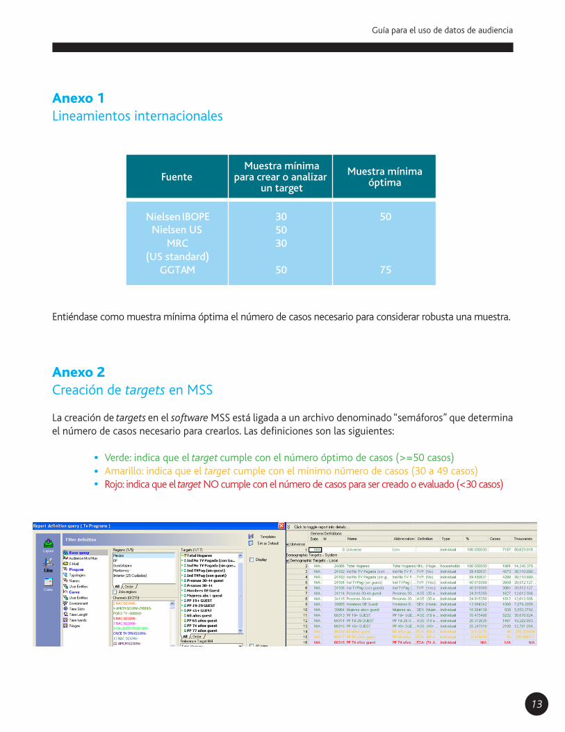
Anexo 1Lineamientos internacionales

Entiéndase como muestra mínima óptima el número de casos necesario para considerar robusta una muestra.

Anexo 2Creación de targets en MSS

La creación de targets en el software MSS está ligada a un archivo denominado “semáforos” que determina el número de casos necesario para crearlos. Las definiciones son las siguientes:

Verde: indica que el target cumple con el número óptimo de casos (>=50 casos)Amarillo: indica que el target cumple con el mínimo número de casos (30 a 49 casos)Rojo: indica que el target NO cumple con el número de casos para ser creado o evaluado (<30 casos)

Fuente

IBOPE

MRC(US standard)

GGTAM

305030

50

50

75

Muestra mínimapara crear o analizar

un target

Muestra mínimaóptima

NielsenNielsen US

14


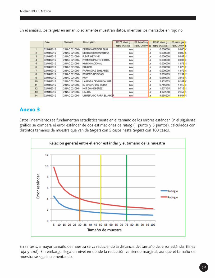
En el análisis, los targets en amarillo solamente muestran datos, mientras los marcados en rojo no:

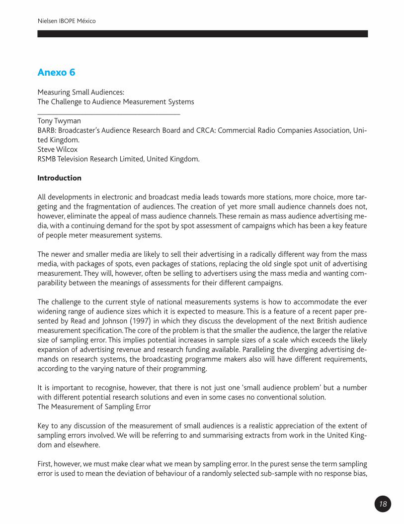
Anexo 3

Estos lineamientos se fundamentan estadísticamente en el tamaño de los errores estándar. En el siguiente gráfico se compara el error estándar de dos estimaciones de rating (1 punto y 5 puntos), calculados con distintos tamaños de muestra que van de targets con 5 casos hasta targets con 100 casos.

En síntesis, a mayor tamaño de muestra se va reduciendo la distancia del tamaño del error estándar (línea roja y azul). Sin embargo, llega un nivel en donde la reducción va siendo marginal, aunque el tamaño de muestra se siga incrementando.

Anexo 4

Relación general entre el error estándar y el tamaño de la muestra

Erro

r es

tánd

ar

Tamaño de muestra

15


En el siguiente gráfico se expone un ejercicio teórico para verificar el mínimo número de casos en muestra que podría ser establecido como óptimo, en torno a los distintos tamaños de ratings que regularmente maneja la industria. ³

Cada línea representa un número de casos en muestra y presenta el comportamiento del error estándar de acuerdo con los diferentes tamaños de rating que van desde 0.1% a 11%. Sobre el análisis:

El recuadro azul enmarca la zona en donde se encuentra 80% de los distintos tamaños de ra-ting de 17 targets (en individuos) que regularmente trabaja la industria³, y la línea roja vertical establece el promedio de dicho 80% (1.8 puntos de rating).La separación entre cada una de las líneas es casi la acumulación de distancia entre sus pre-cedentes respecto sus consecuentes. Se ilustran dos distancias: entre la línea azul fuerte (500 casos) y la morada (200 casos) hay una distancia de error determinada por la disminución de 300 casos en muestra (A). Dicha distancia en error es ligeramente menor a la distancia esta-blecida entre la línea morada (200 casos) a la azul clara (100 casos) (B). Cuando se entiende que la disminución en muestra es sólo de 100 casos, es decir, un tercio de disminución de muestra respecto la establecida en (A). Este fenómeno resulta en errores más significativos a medida que se reduce el tamaño de muestra y se llega a casos como 50 y 30 casos.

Este ejercicio explica que respecto a los tamaños de rating con los que actualmente trabaja la industria (recuadro azul), targets de entre 200 y 500 casos podrían considerar un error estándar muy cercano, lo cual

Tamaño de la muestra

Error estándar

Tamaño del rating %

0.0%

1.0%

2.0%

3.0%

4.0%

5.0%

6.0%

0.1% 0.5% 1.0% 3.0% 5.0% 7.0% 9.0% 11.0%

500 400 300 200 100 50 30

AV1.8

80% del os ra ngs%

50

100

200

300

30

400500

A

B

AV1.8

s%

Punt

os d

irec

tos

de ra

ting

%

AVG1.8

80% de los ratings%

Anexo 4

16


contribuiría a dar mayor certidumbre acerca de análisis “puntuales”; es decir, consulta diaria y franjas en minutos. Cuando se trabaja con menos de 200 casos, y en especial con menos de 100, los errores estándar serán más significativos dado que los tamaños de muestra no actúan proporcionalmente.

³Tamaño de rating por minuto de enero 1 a septiembre 20 de 2012, en los targets personas total con guest, personas 19+ con guests, personas 19+ sin DE con guest, personas 4-12 con guests, amas de casa, mujeres ABC+C 19-44 con guest, mujeres CD+ 19-44 con guest, hombres ABC+C 19-44 con guest, hombres CD+ 19-44 con guest, personas ABC+C 19-44 con guest, personas CD+ 19-44 con guest, amas de casa ABC+C, amas de casa CD+, personas 4-12 ABC+C con guest, personas 4-12 CD+ con guest, personas 13-18 ABC+C con guest, personas 13-18 CD+ con guest; canales Proyecto 40; Cadena Tres; C2; C5; C7; C9; C13; TVP; foro tv. Total 28 ciudades.

17


Anexo 5

Se realizó un ejercicio de simulación de rotación del panel que consideró a todos los hogares intab del 1 de enero al 30 de junio de 2012 (6 meses de datos). En cada base diaria fue reemplazado el número de identificación de 20 hogares, por ejemplo, en la base del día 1 de enero se reemplazó el identificador de 20 hogares, el día 2 de enero se cambiaron los 20 del día 1 de enero más otros 20 nuevos, y así sucesivamente hasta cambiar el identificador de todos los hogares del panel hasta el último día de junio.

Una vez ejecutados estos cambios de identificador de hogares, se calculó el Alcance y Frecuencia de varias campañas publicitarias de distintos sectores cuya duración fuera de un mes, otra de tres meses y una última de seis meses. Asimismo, se calcularon los datos en 17 targets personas², los más utilizados por la industria.

Los resultados obtenidos derivaron los siguientes resultados -en promedio- de todos los targets consulta-dos, como se muestra en los siguientes gráficos:

Es importante mencionar que la razón del decremento en Alcance e incremento en Frecuencia se genera por la forma en que se construyen las matrices de panel continuo dentro de su cálculo. Para cada caso en muestra se determina un expansor ponderado con base en la continuidad que cada uno tiene en el periodo de análisis seleccionado.

Decremento del Alcancepor la rotación

Aumento de la Frecuenciapor la rotación

18


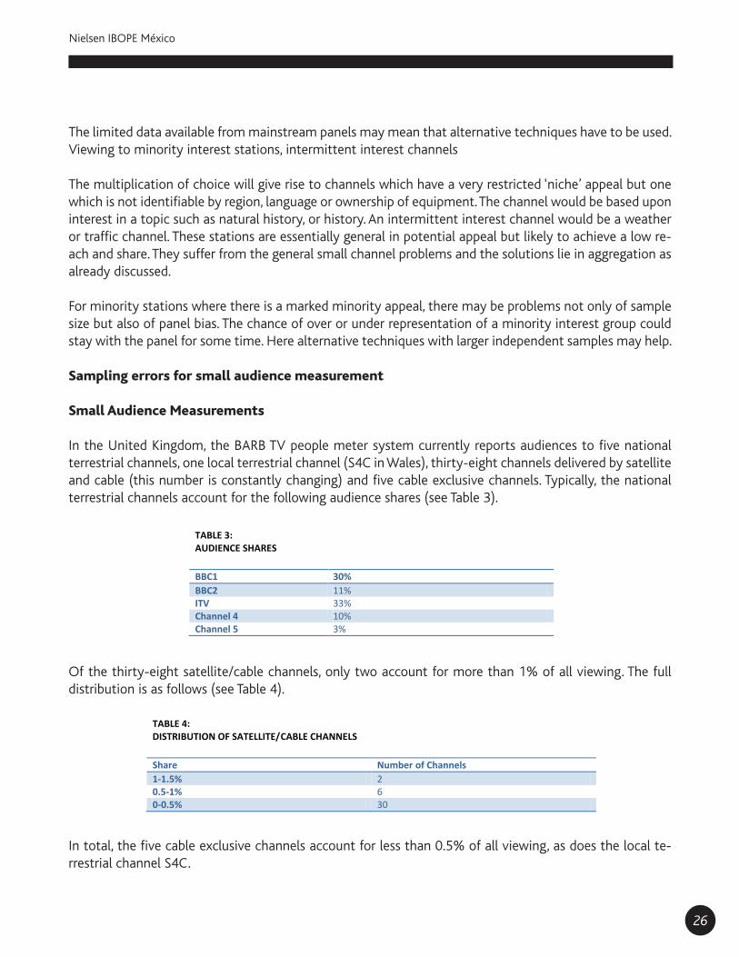
Anexo 6

Measuring Small Audiences:The Challenge to Audience Measurement Systems________________________________________Tony TwymanBARB: Broadcaster’s Audience Research Board and CRCA: Commercial Radio Companies Association, Uni-ted Kingdom.Steve Wilcox RSMB Television Research Limited, United Kingdom.

Introduction

All developments in electronic and broadcast media leads towards more stations, more choice, more tar-geting and the fragmentation of audiences. The creation of yet more small audience channels does not, however, eliminate the appeal of mass audience channels. These remain as mass audience advertising me-dia, with a continuing demand for the spot by spot assessment of campaigns which has been a key feature of people meter measurement systems.

The newer and smaller media are likely to sell their advertising in a radically different way from the mass media, with packages of spots, even packages of stations, replacing the old single spot unit of advertising measurement. They will, however, often be selling to advertisers using the mass media and wanting com-parability between the meanings of assessments for their different campaigns.

The challenge to the current style of national measurements systems is how to accommodate the ever widening range of audience sizes which it is expected to measure. This is a feature of a recent paper pre-sented by Read and Johnson (1997) in which they discuss the development of the next British audience measurement specification. The core of the problem is that the smaller the audience, the larger the relative size of sampling error. This implies potential increases in sample sizes of a scale which exceeds the likely expansion of advertising revenue and research funding available. Paralleling the diverging advertising de-mands on research systems, the broadcasting programme makers also will have different requirements, according to the varying nature of their programming.

It is important to recognise, however, that there is not just one ‘small audience problem’ but a number with different potential research solutions and even in some cases no conventional solution.The Measurement of Sampling Error

Key to any discussion of the measurement of small audiences is a realistic appreciation of the extent of sampling errors involved. We will be referring to and summarising extracts from work in the United King-dom and elsewhere.

First, however, we must make clear what we mean by sampling error. In the purest sense the term sampling error is used to mean the deviation of behaviour of a randomly selected sub-sample with no response bias,

19


from the behaviour of the total population. Practical situations are far from this. Samples are not purely random and there is response bias but we still need to understand the variability of the data.In using the term ‘sampling error’ we want to express the degree of variability which any measurement or comparison between measurements is subject to when there is no real change in the behaviour which it is intended to measure.

With panels there are a number of factors which contribute to the amount of statistical variability:

When panels are initially recruited, the sample will be biased through:differential non-response biases inherent in the system, chance features of the particular sam-ple selected which remain as a sample bias, changing over time as panel membership changes.Comparisons between measurements at different times involves many of the same individuals and according to the degree of correlation between their behaviour at those times, there is a reduction in sampling error. This correlation diminishes over time, however, as people get older, change their social life, their work life and their interests.The need to balance known demographic imbalances involves weighting which can signifi-cantly decrease effective sample size and increase sampling error.

Types of Small Audience Situations

In this paper we seek to identify the range of small audience situations, the likely data requirements and how they might be researched. We are not starting with a ‘clean slate’ here. In most countries with broad-casting systems sufficiently developed to generate small station problems there will already be sophisti-cated people meter systems.

These have been designed initially to measure mass audiences but have been progressively expanded and adapted to report on smaller audiences. Research solutions have to be considered:

within existing systems,by expanding and adapting existing systems,by creating entirely new research sources.

Viewing by Smaller Sub-Groups to Larger Stations

This is essentially a problem of sample size. Viewing by smaller sub-groups to larger stations is a situation which regularly occurs within existing systems and even for mass audience channels. There appears to be a law whereby, whatever the sample size, the number of sub-groups reported expands to include many for which the sample size is inadequate.

Within the current BARB system the sample sizes and sampling errors shown in Table 1 for the largest regional panel illustrate the point.

20


These sampling errors assume the panel to be perfectly balanced. In reality the sampling errors are up to 20% larger for the actual panel which is weighted to correct for demographic profile imbalances. So these sampling errors represent the best that could be achieved given the total number of homes available. It is salutary to note that these sampling errors are for a peak time rating on the largest commercial TV station in the United Kingdom.

Any attempt at optimising the choice of individual spots on the smaller sub-groups is clearly a waste of time.

One common response to statistics such as these is that practices should change and that trading should be based on larger more reliable sub-groups and/or that optimisations and appraisal should be in terms of schedules rather than individual spots. The statistical reliability of this approach is discussed in a later section.Another approach under test in the United Kingdom for regional sub-groups is that of modelling or fac-toring from the network panel.

The principle is that a regional panel measures the main audience categories directly. Sub-group audiences are then factored by applying the relationship between the sub-group and the main category found at that time on the larger network panel, to the directly measured regional main category audience. This factor is derived after weighting the network data to match the demographic profile of the region. A summary of this is provided in a later section.

This approach can be used to reduce sub-group variability equivalent to increasing effective sample size by between 50% and 100%. This is an increase beyond the levels of affordability, but even that is not enough where the market is trying to trade on sub-groups with samples of fifty.

This approach we believe could be used in the United Kingdom and help to make sub-group data more reliable. It is, however, viable only in conditions such as in the United Kingdom where there is a broad fra-mework of consistency in programming across the regions within the network and few marked deviations of programming style at the regional level. We have not found evidence that regional variations in pro-

TABLE 1: SAMPLE SIZES AND SAMPLING ERROR

S ample Size TVR Interval

All Individuals Adults Men Women Housewives

1204 996 459 537 530

9.6 11.1 11.0 11.2 12.7

+ 24% + 22% + 28% + 26% + 22%

Housewives with Children Women ABC1 Men 16-34

154 296 164

9.8 8.9 5.9

+ 49% + 42% + 70%

Women AB Men 16-24 Children

129 62 208

4.8 7.8 2.5

+ 88% + 88% + 105%

8:30pm

21


gramming do affect the validity of factoring.

Factoring, however, applies most readily to a regional panel structure for mass audiences. It is no solution for small area channels like cable or niche channels. Overall our solution to small sub-group audiences on larger panels is to suggest that the sampling errors should be examined (as above), samples increased to what is affordable and to accept that trading on spots for those sub-groups which cannot be measured reliably will be unproductive.

Steps which can help are trading and appraisal in terms of schedules of spots and in appropriate cases, factoring.

Viewing by Large Sub-Groups to Smaller Stations or Large Stations at Off-Peak TimesPut more simply this is the problem of small ratings on large panels. As competition increases, audiences fragment and there are always:

stations which always have low ratings,times when even large stations have low ratings.

This situation occurs increasingly within panels designed to measure mass audiences. Where stations are restricted by access such as for satellite or cable, panels representative of those sub-sections of the uni-verse can be recruited.

In the United Kingdom, homes with satellite or cable are broken out of the main panel and weighted as a network satellite panel. This provides around 1200 households and 3600 individuals, without any additio-nal boosting.

Such is the fragmentation within these homes however, that many stations record permanently low wee-kly audiences. These data are robust within satellite homes for the terrestrial channels, for total Sky and other aggregations of channels. Some channels, however, regularly record an average of one or two minu-tes of viewing per head each week. In a sense these figures are reliable in that they always show very low audiences week after week.

Where the problems arise, for all channels, is when individuals spots or programmes are considered. For many of the larger satellite stations, even within the satellite universe, many ratings at individual times are 1% or less, often 0.1% or less.

The sampling errors on these are enormous. For example, consider the largest satellite channel in the Uni-ted Kingdom. Amongst all housewives this channel took a 4.5% share of all viewing in satellite receiving homes in a recent week (week ending 25th January 1998). (Note that the next largest satellite channel took only a 2.6% share.) In this particular week, two-thirds of this channel’s programmes had housewife ratings of 1% or less and one-third had housewife ratings of 0.1% or less. The 95% confidence intervals on housewife ratings of 1% and 0.1% in satellite homes are 60% and 180% respectively. (Again these sampling errors assume the panel to be perfectly balanced; in reality they are larger.)

22


Two-thirds of the satellite channels reported by BARB never achieved any rating as high as 1% in this particular week.If audiences are expressed in terms of numbers of viewers, however, they take on a reality which belies their statistical bias. For example, a programme with a rating of 0.5% could easily lose all its audience from one week to the next purely as a result of sampling error. Amongst housewives in satellite homes (there are 6.6 million in the population) this represents a drop in the audience from over 30,000 to nothing at all. How can you lose 30,000 viewers from one week to the next? Because they represent small ratings with big sampling errors, the variability looks implausible.

What is the solution? This depends on the purpose for which audience research data are needed.Programming: it is certainly possible to see which are the most successful programmes even from highly unstable small ratings data for small stations. Judgement is considerably improved by managing several weeks data together.

The precision of assessment for programme audiences is less than for large rating channels but the need for more subtle distinctions may be less. The differences between programmes may even become more deviant because they may be less affected by competition.

Buying and selling advertising: here any attempt to work on an individual spot time may be a waste of time. Improved assessments may be made by:

using data averaged over time,assessing whole schedules either within a channel but more realistically across a number of channels.

For advertisers on niche channels representing a special market, e.g. a computer channel, advertisers may well wish to get an idea of the best times to advertise. They are, however, more likely to buy a schedule and compare the direct response with campaigns in other media. It is possible that the more specialised the market, the less precise audience estimates are required.

Viewing to stations with restricted universes

With panels covering the whole television universe, some restricted universes may be represented with only small sample sizes and there may be difficulties in representing their characteristics. Restricted uni-verses in this sense occur in a number of ways.

Limited regional coverage

In the United Kingdom some cable franchises have small catchment areas. Within BARB, cable as a whole is represented by a panel which is a specially weighted sub-set of the main panels. This reports separately on cable stations which have a wide geographical coverage. Small regional cable franchises may, however, wish to know the patterns of viewing to the station mix which they offer and their own local cable servi-ces. Their coverage by a network people meter sample is negligible. It would be possible but not economi-cally viable to recruit a special people meter panel for the area. Instead, in the United Kingdom, the Cable

23


Research Group have commissioned, outside BARB, periodic two-week paper diary studies using diary formats not unlike those used for much radio research. Some of this work is described in a later section. This kind of situation is likely to increase for the future.

Most regional television structures end up with regions that vary in size. This often means that the smaller stations would not have an adequate sample based upon proportionate regional sampling. The solution is usually disproportionate geographical sampling or a federation of regional panels.

Whilst strict statistical logic would demand equal sized panels everywhere the money at risk argument often leads to compromise whereby larger areas may be capped off at a certain limit and smaller areas boosted up. The United Kingdom is an example of this illustrated by three of the thirteen regional areas (see Table 2).

One of the problems is that there is sometimes a tendency to treat all the areas as having the same cu-rrency available. Thus the sample size for Border hardly warrants pursuit of spot by spot buying, certainly not for sub-groups, but it sometimes happens. Possible remedies include selling by schedules or aggrega-ted ratings and factoring discussed elsewhere.

An example of equal sized regional panels is Belgium with two equal panels of 750 households for each of the Flemish and French speaking parts. Paradoxically, although the national sample is about a third of the United Kingdom’s, the actual panels used for trading are larger. A regional programming and trading structure is one situation where, even with mass audience channels, the use of people meter panels leads to statistical strain. It seems likely, however, that there is a general trend towards trading television adver-tising in larger units which may ease this.

Services based upon new technology

The advent of satellite transmissions was a past example of this. There it was possible to recruit a special sample of satellite receivers who had a vastly increased range of programme choice compared with te-rrestrial reception. In the United Kingdom there was initially a separate panel but ultimately a specially weighted sub-sample of the main people meter panels was used. This currently provides a sample of around 1200 households.

We expect that digital television will be measured in the same way in the United Kingdom. This could ini-tially involve special extra panels for satellite digital, terrestrial digital and even digital cable services since

TABLE 2: EXAMPLE OF REGIONAL AREAS WITHIN THE UNITED KINGDOM

Percent of Meters Sample Size Households

London 20.2% 11.7% 525 North East 5.3% 6 .1% 275 Border 1.2% 2.2% 100

24


there is very likely to be much initial overlap between this mode of reception. Such panels could be merged with analogous panels when the universe is large enough.

These new developments present special small audience problems:

a. Universes. It is easy to define access to equipment but harder to measure it when it starts from zero and may rise rapidly and erratically. Within the broadest definition of having the reception equipment, however, there is the added complication of subscription packages in-corporating different channels. These are subject to an additional variability from take-up and churn within the variability of the equipment universe. Universes have been generally obtai-ned from some independent survey source. An establishment survey, for example, for a slowly changing terrestrial source can provide:

a reliable estimate of universe size,a profile of demographic and often characteristics of the universe,a source of households for panel recruitment.

With new services such as digital transmissions the new problems are that the universes are:initially very small,dispersed through the population,changing very rapidly; for individual stations up and down,highly complex in terms of combinations of channels received.

These characteristics mean that no representative sample is likely to be large enough, afforda-ble on a continuous basis nor even able to be processed quickly enough. This means that some alternative approach is necessary. In practice broadcasters will have exact databases showing who is paying for and receiving what on a near-daily basis. It would be logical to use this. The objection is sometimes raised that broadcasters might inflate the figures and/or be able to detect the identity of the panel home. It will be necessary to counter this by some form of independent auditing and access to the database. It will also be necessary to create new legal safeguards and protection against interference with panel homes. The use of a broadcaster’s database does not uniquely create this problem, it is there from the moment that the broad-caster gets into a direct one-to-one on-going relationship with the households in the audience.Ultimately intelligent digital decoders will be able to record station viewing data in great detail on large samples. This will need some individual viewing data from smaller samples modelled onto it. This would solve both the universe and the small audiences problem for marketing strategies based on type of household rather than type of individual.

b. Audience fragmentation. New technologies bring more choice and greater fragmenta-tion. Digital television is likely to extend the range of channels from the thirty or more of satellite into the hundreds. Different channels will show the same films at different times to provide a near video-on-demand service. Necessarily, most audiences will be very small, a further extension of the issues discussed earlier. This means that for all but a few channels the assessment of individual spot ratings will be pointless. We would expect to see television planning and assessment based upon aggregated data probably involving selling of schedules comprising many small ratings spread across a range of channels.

25


Once again the receiving of schedule audience measurement becomes of crucial importance.

c. Panel structure. As services develop those which can afford people meter panels will pro-bably do so but initially, with relatively small sample sizes. It will also be necessary to control panel membership in terms of:

combinations of channels received,novelty effects, i.e. length of ownership.

This will require complex weighting reducing effective sample sizes even more and exacerba-ting the problems of fragmentation discussed above. Only data aggregated across channels and/or times will be robust.

When choice gets this complex and with the development of electronic programme guides where pro-grammes can be chosen without channel awareness, the option of using alternative techniques such as paper diaries and recall will no longer exist.

The industry will therefore have to get used to using audience measurement data for small audiences from small people meter panels in a responsible way using aggregated data. Until that is the intelligent decoder is able to give precise set range data on large samples.

Programming needs will vary according to the nature of the channel. Even with very small share channels it is possible to see which are the most popular programmes, particularly if schedules are consistent and weeks averaged together. BARB currently publishes Programme Top Tens for many small share channels, which are robust, in the sense of similar programmes appearing week after week. Any subtlety in terms of small differences between audiences would, however, be impossible. Programmers wishing to fine tune programmes or schedules would probably gain more from qualitative research among viewers to their programmes.

Ethnic or language minorities

Ethnic or minority language groups are likely, by definition, to have low representation on general repre-sentative samples. There are likely to be special sampling problems in that such groups are both clustered but not exclusively confined within any geographical boundary. Universe measurement and sample selec-tion probably requires large scale surveys and some allowance made for differential non response. Even then the sample may not be adequate to provide reliable data for channels servicing these groups.

One solution is a separate people meter panel. This occurs in the United Kingdom for Welsh speakers, measuring audiences to S4C. There is no separate panel for Gaelic speakers in Scotland. Response to pro-grammes in Gaelic is studied through qualitative audience appreciation studies. The Gaelic channel in the Republic of Ireland has Gaelic speakers as a possible audience sub-group on the main panel. In Germany foreigners have been excluded from the main television panel universes but may now be represented by a separate panel.

Whether an ethnic minority or language channel has a separate panel is largely a matter of economics.Cable and the development of digital services will make niche channels possible for smaller ethnic groups.

26


The limited data available from mainstream panels may mean that alternative techniques have to be used.Viewing to minority interest stations, intermittent interest channels

The multiplication of choice will give rise to channels which have a very restricted ‘niche’ appeal but one which is not identifiable by region, language or ownership of equipment. The channel would be based upon interest in a topic such as natural history, or history. An intermittent interest channel would be a weather or traffic channel. These stations are essentially general in potential appeal but likely to achieve a low re-ach and share. They suffer from the general small channel problems and the solutions lie in aggregation as already discussed.

For minority stations where there is a marked minority appeal, there may be problems not only of sample size but also of panel bias. The chance of over or under representation of a minority interest group could stay with the panel for some time. Here alternative techniques with larger independent samples may help.

Sampling errors for small audience measurement

Small Audience Measurements

In the United Kingdom, the BARB TV people meter system currently reports audiences to five national terrestrial channels, one local terrestrial channel (S4C in Wales), thirty-eight channels delivered by satellite and cable (this number is constantly changing) and five cable exclusive channels. Typically, the national terrestrial channels account for the following audience shares (see Table 3).

Of the thirty-eight satellite/cable channels, only two account for more than 1% of all viewing. The full distribution is as follows (see Table 4).

In total, the five cable exclusive channels account for less than 0.5% of all viewing, as does the local te-rrestrial channel S4C.

TABLE 3: AUDIENCE SHARES

BBC1 30% BBC2 11% ITV 33% Channel 4 10% Channel 5 3%

TABLE 4: DISTRIBUTION OF SATELLITE/CABLE CHANNELS

Share Number of Channels 1-1.5% 2 0.5-1% 6 0-0.5% 30

27


A large number of cable exclusive channels are not reported by the BARB system because the data is not considered to be sufficiently robust. (These are catered for outside the BARB system.) The arrival of digital TV later this year will generate yet another small audience measurement requirement.

The small channel shares are partly due to the large numbers of channels available and partly because only 34% of the population have access to cable or satellite and only 13% are cable exclusive.

In the United Kingdom, the national terrestrial channels are also commonly reported on a regional basis, in terms of either the twelve BBC editorial regions or sixteen ITV areas. This is another key dimension resulting in small audiences. For example, if 10% of the population live in a particular ITV area, then the share of all TV viewing by the whole national population which is accounted for by viewing to the ITV station broadcasting in that area is only 3.3% (i.e. 10% of the national ITV share of 33%). Effectively this is another example of a restricted availability channel because only 10% of the population has access to that particular regional ITV station.

The last dimension which results in audience fragmentation is the need to report on demographic ca-tegories, ranging from simple male/female splits to very tightly defined age groups. For example, a 10% penetration sub-group’s viewing to an ITV station in an area containing 10% of the population would only account for 0.33% of the total national populations’ viewing.

Of course it is not normal practice to report such fragmented audiences as percentages of the total natio-nal population base. Therefore the percentages are not normally seen as such small numbers. However, this way of presenting the audiences is a useful lead in to the consideration of sampling errors and the relative reliability of the various audience measurements.

Sampling Error Study

BARB and RSMB have recently completed the first phase of a major study of the sampling errors asso-ciated with the various audience measurements produced by the TV people meter panel in the United Kingdom. This is considered to be an essential contribution to the sample design component of the future audience measurement specification. The theory has been developed to allow the calculation of sampling errors for many different audience measurements and to compare the performance of perfectly balanced proportionate and disproportionate designs and to assess the effect of weighting used to correct for the usual panel imbalances that exist within an operational system.

The calculation of sampling error

Several papers have been written concerning the components of sampling error and the methodology for their calculation (eg. Schillmoeller, 1992; Boon, 1994 and Twyman and Wilcox, 1996).

The calculation of sampling error takes account of the variability in the audience measurement between individuals, the sample size, clustering within households and weighting. These factors and their effects can be different for each measurement, for each channel, for each demographic category and each area base.

28


It was necessary to consider the whole range of different audience measurements because some will have smaller sampling errors than others and therefore may be more useful in the small audience situation:

average ratings and channel share for all-time, time segments (day-parts), quarter hours and individual minutes;channel reach;programme, commercial break and individual commercial spot ratings;reach and frequency analysis;daily, weekly and four week averages;change over time, from month to month and from year to year.

The actual analyses were based on a limited number of channels using two ITV area panels. For the purpo-ses of this paper, the results have been interpreted to provide approximate sampling errors for a number of hypothetical situations.

All sampling errors have been converted to 95% confidence intervals. This means there is a 5% chance that the audience measurement estimate is more than one confidence interval from the ‘true’ value of the audience measurement.

Sampling errors for proportionate panel designs

Because network based channel share encapsulates the extent of each small audience situation, a useful start point is to consider the sampling errors on channel shares for the types of viewing situations descri-bed in earlier.

Sampling errors have not yet been calculated for Channel 5, S4C nor any of the cable channels so inter-polations have been made. It should also be noted that sampling errors have not been calculated for any

TABLE 5: CHANNEL SHARE SAMPLING ERRORS - ALL ADULTS 16+, NETWORK

Channel Share Single Minute Single Day 4 Week Average BBC 1 30.0% + 10 % + 1.4% + 0.9% BBC 2 11.0% + 19% + 2.3% + 1.2% ITV 33.0% + 9% + 1.2% + 0.8% Channel 4 10.0% + 20% + 2.1% + 1.2% Channel 5* 3.0% + 30% + 5% + 3% Satellite 1.0-1.5% + 50% + 8% + 5% Satellite 0.5-1.0% + 65% + 10% + 6% Satellite* Under 0.5% + 90% + 15% + 8% S4C* 0.3% + 90% + 15% + 8% Cable only* Under 0.25% + 100% + 20% + 10% Sampling errors have not yet been calculated for Channel 5, S4C nor any of the cable channels so

calculated for any satellite channels with less than 0.1% share. The single minute sampling error relates to peak-

29


satellite channels with less than 0.1% share. The single minute sampling error relates to peak-time.

The BARB panel in the United Kingdom is currently nearly 4500 homes with 8600 adults. If this were to be of a proportionate design and perfectly balanced (i.e. no weighting were required) then the shares of viewing would have the following sampling errors. These are shown for a single minute, a single day and then for a four week average in Table 5.

At the next level of fragmentation (see Table 6), consider sampling errors for an average 10% penetration demographic sub-group or a 10% penetration geographical region. The network based channel shares are all divided by ten. The sampling errors above increase as the sample size decreases - i.e. multiply by .

For highly targeted channels this table must be interpreted carefully. This is because it would not be nor-mal practice to analyze ‘average’ demographic sub-groups. More often than not the key target sub-group would account for a large proportion of the channel’s total audience. In this situation the percentage sampling error will not increase as much as the decrease in sample size suggests because the sub-group has higher viewing levels. In fact we can hypothesis that if we do have a situation where the whole of a channel’s audience is attributed to one key demographic sub-group (e.g. 16-34 year olds and a ‘young’ music channel) then the percentage sampling error for the sub-group is the same as for all adults.

This can be demonstrated theoretically, using single minute ratings rather than channel share in order to keep things simple:

Network sample = 8600 adultsSingle minute TVR = 1Sampling error =

95% confidence interval = 0.214 = 21%Now suppose that the whole of this audience is contained within a 10% penetration sub-group. Then:

TABLE 6 CHANNEL SHARE SAMPLING ERRORS - 10% SUB-GROUP OR REGION

Channel Share Single Minute Single Day 4 Week Average BBC1 BBC2 ITV Channel 4 Channel 5* Satellite Satellite Satellite* Cable only*

3.0% 1.1% 3.3% 1.0% 0.3% 0.10-0.15% 0.05-0.10% Under 0.05% Under .025%

+ 32% + 61% + 29% + 64% + 96% + 160% + 208% + 288% + 320%

+ 4% + 7% + 4% + 7% + 16% + 25% + 32% + 47% + 63%

+ 3% + 4% + 3% + 4% + 9% + 16% + 19% + 25% + 32%

30


Sub-group sample = 860 adultsSingle minute TVR = 10Sampling error =

95% confidence interval = 2.04 = 20% which is almost exactly the same and therefore almost totally independent of the sample size.

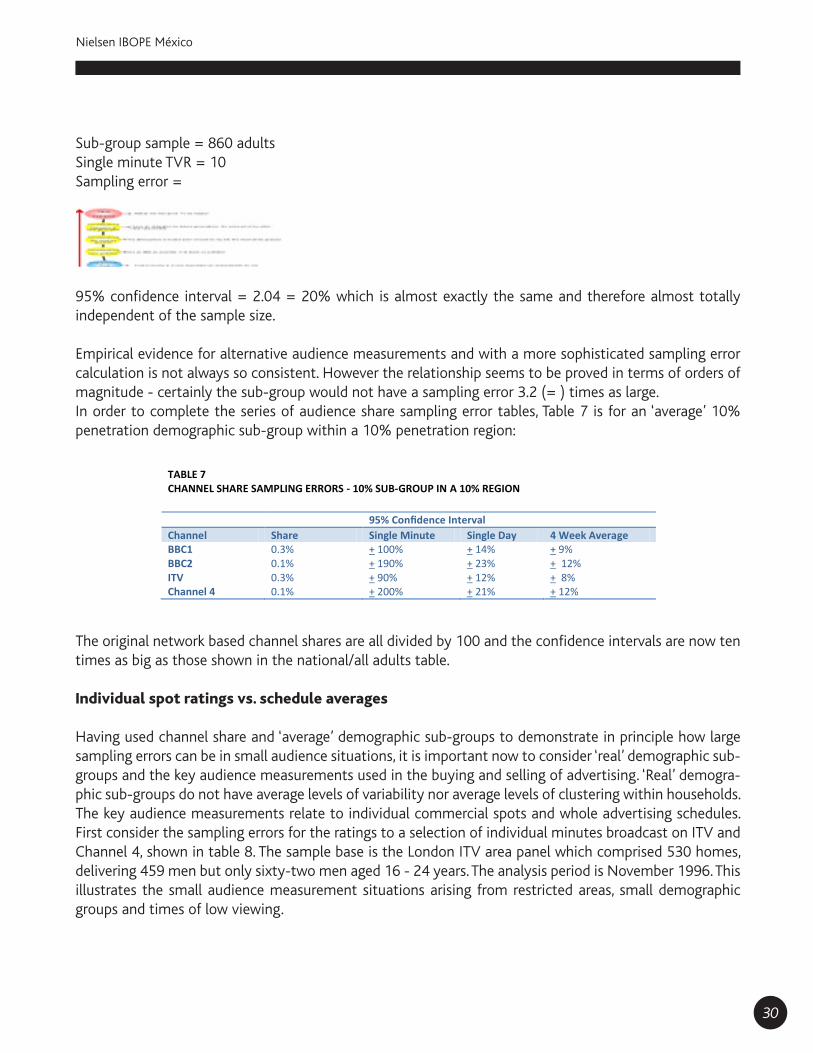
Empirical evidence for alternative audience measurements and with a more sophisticated sampling error calculation is not always so consistent. However the relationship seems to be proved in terms of orders of magnitude - certainly the sub-group would not have a sampling error 3.2 (= ) times as large.In order to complete the series of audience share sampling error tables, Table 7 is for an ‘average’ 10% penetration demographic sub-group within a 10% penetration region:

The original network based channel shares are all divided by 100 and the confidence intervals are now ten times as big as those shown in the national/all adults table.

Individual spot ratings vs. schedule averages

Having used channel share and ‘average’ demographic sub-groups to demonstrate in principle how large sampling errors can be in small audience situations, it is important now to consider ‘real’ demographic sub-groups and the key audience measurements used in the buying and selling of advertising. ‘Real’ demogra-phic sub-groups do not have average levels of variability nor average levels of clustering within households. The key audience measurements relate to individual commercial spots and whole advertising schedules. First consider the sampling errors for the ratings to a selection of individual minutes broadcast on ITV and Channel 4, shown in table 8. The sample base is the London ITV area panel which comprised 530 homes, delivering 459 men but only sixty-two men aged 16 - 24 years. The analysis period is November 1996. This illustrates the small audience measurement situations arising from restricted areas, small demographic groups and times of low viewing.

TABLE 7 CHANNEL SHARE SAMPLING ERRORS - 10% SUB-GROUP IN A 10% REGION

Channel Share Single Minute Single Day 4 Week Average BBC1 BBC2 ITV Channel 4

0.3% 0.1% 0.3% 0.1%

+ 100% + 190% + 90% + 200%

+ 14% + 23% + 12% + 21%

+ 9% + 12% + 8% + 12%

31


All the sampling errors are large, even for the peak-time ITV All Men rating. The sampling error for men aged 16-24 years is huge. The zero Channel 4 ratings actually emphasise the small sample problem - even a Men 16-24 rating of 5% (as achieved within All Men) would be the result of only three individual panel members viewing.

By averaging over time, even within a continuous panel, there will be significant reductions in sampling error. This fundamental theory originally expounded in a report prepared by Arbitron (1974) has been de-monstrated in several published papers (e.g. Wilcox and Reeve, 1992). For example, average ratings over four consecutive Mondays have the sampling errors shown in Table 9.

TABLE 8: SAMPLING ERRORS FOR INDIVIDUAL MINUTE RATINGS

Channel Time A ll Men M en 16-24 TVR 95% c.i. TVR 95% c.i. ITV 7:45am

1:45pm 8:30pm

1.3 5.1 11.0

+ 39% + 21% + 14%

2.5 3.8 7.8

+ 95% + 68% + 44%

CH4 7:45am 1:45pm 8:30pm

0.5 0.4 5.0

+ 81% + 77% + 23%

0.0 0.0 0.0

- - -

TABLE 9: SAMPLING ERRORS FOR AVERAGE RATINGS - FOUR MONDAYS

Channel Time A ll Men Men 16-24 TVR 95% c.i. TVR 95% c.i. ITV 7:45am

1:45pm 8:30pm

1.2 3.5 13.2

+ 24% + 15% + 5%

1.6 2.1 7.1

+ 57% + 45% + 19%

CH4 7:45am 1:45pm 8:30pm

0.4 1.0 3.1

+ 39% + 13% + 10%

0.1 0.4 1.3

+ 88% + 43% + 33%

32


Although there is some variability in the relationship with the single minute rating sampling errors - to be expected with real data and small samples - on average the percentage sampling errors are halved. We believe that many broadcasters are already using such averages for planning purposes.

This principle can be extended to whole schedules where in general we will find even greater reductions in sampling errors. Table 10 shows results for five schedules broadcast in November 1996, again based upon the London panel.

For All Men and for any schedule with a reasonable number of ratings, the sampling errors have reduced to a more manageable level. However, there does seem to be a plateau beyond which additional ratings will not result in further sampling error reductions. For All Men the minimum 95% confidence interval seems to be 5% whilst for Men 16-24 it is about 15%. This is approximately in line with their relative sample sizes although Men 16-24 are also more variable as a group.

However, the basic principle is clearly demonstrated: schedule total ratings have much smaller sampling errors than do individual commercial spot ratings.

Sampling errors for different schedule structures

A key question we have asked is how much the sampling error for schedule total ratings is dependent upon the composition of the schedule, i.e. is the schedule total ratings percentage sampling error high if the indi-vidual spots in the schedule have low ratings and therefore high percentage sampling errors? For example, is the sampling error for a schedule of ten spots with an average rating of 20% the same as for a schedule of twenty spots with an average rating of 10%? The principle can be demonstrated with some simplistic theory.

TABLE 10: SAMPLING ERRORS FOR TOTAL SCHEDULE RATINGS

Schedule C hannel A ll Men Men 16-24 Total TVRs 95% c.i. Total TVRs 95% c.i. I ITV

Channel 4 Satellite Total

33 19 4 55

+ 15% + 18% + 26% + 12%

39 15 2 56

+ 25% + 51% + 67% + 29%

II ITV Channel 4 Satellite Total

148 71 14 233

+ 6% + 9% + 18% + 5%

87 54 16 157

+ 19% + 24% + 52% + 16%

III ITV Channel 4 Satellite Total

140 36 10 186

+ 7% + 9% + 19% + 6%

116 28 28 173

+ 18% + 24% + 33% + 15%

IV ITV Channel 4 Satellite Total

254 171 36 461

+ 6% + 6% + 17% + 5%

134 148 55 337

+ 20% + 21% + 28% + 15%

V ITV Channel 4 Satellite Total

174 64 17 256

+ 7% + 9% + 20% + 6%

88 32 21 141

+ 26% + 29% + 58% + 21%

33


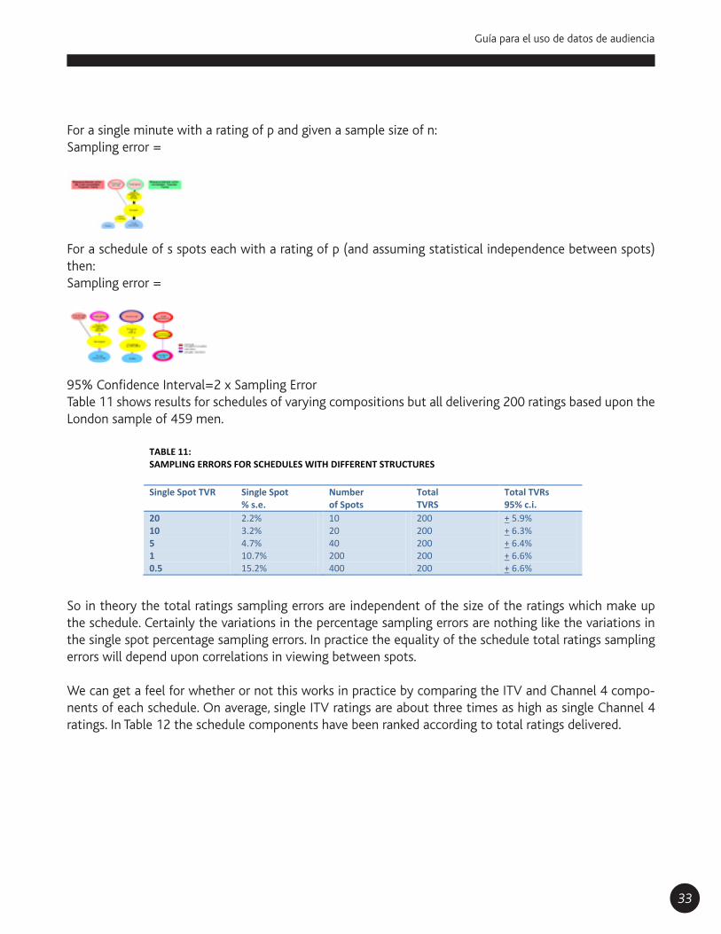
For a single minute with a rating of p and given a sample size of n:Sampling error =

For a schedule of s spots each with a rating of p (and assuming statistical independence between spots) then:Sampling error =

95% Confidence Interval=2 x Sampling ErrorTable 11 shows results for schedules of varying compositions but all delivering 200 ratings based upon the London sample of 459 men.

So in theory the total ratings sampling errors are independent of the size of the ratings which make up the schedule. Certainly the variations in the percentage sampling errors are nothing like the variations in the single spot percentage sampling errors. In practice the equality of the schedule total ratings sampling errors will depend upon correlations in viewing between spots.

We can get a feel for whether or not this works in practice by comparing the ITV and Channel 4 compo-nents of each schedule. On average, single ITV ratings are about three times as high as single Channel 4 ratings. In Table 12 the schedule components have been ranked according to total ratings delivered.

TABLE 11: SAMPLING ERRORS FOR SCHEDULES WITH DIFFERENT STRUCTURES

Single Spot TVR Single Spot % s.e.

Number of Spots

Total TVRS

Total TVRs 95% c.i.

20 10 5 1 0.5

2.2% 3.2% 4.7% 10.7% 15.2%

10 20 40 200 400

200 200 200 200 200

+ 5.9% + 6.3% + 6.4% + 6.6% + 6.6%

34


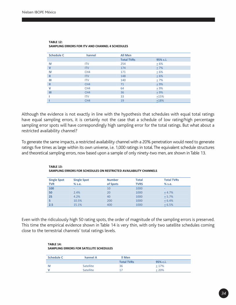
Although the evidence is not exactly in line with the hypothesis that schedules with equal total ratings have equal sampling errors, it is certainly not the case that a schedule of low rating/high percentage sampling error spots will have correspondingly high sampling error for the total ratings. But what about a restricted availability channel?

To generate the same impacts, a restricted availability channel with a 20% penetration would need to generate ratings five times as large within its own universe, i.e. 1,000 ratings in total. The equivalent schedule structures and theoretical sampling errors, now based upon a sample of only ninety-two men, are shown in Table 13.

Even with the ridiculously high 50 rating spots, the order of magnitude of the sampling errors is preserved.This time the empirical evidence shown in Table 14 is very thin, with only two satellite schedules coming close to the terrestrial channels’ total ratings levels.

TABLE 13: SAMPLING ERRORS FOR SCHEDULES ON RESTRICTED AVAILABILITY CHANNELS

Single Spot TVR

Single Spot % s.e.

Number of Spots

Total TVRS

Total TVRs % s.e.

100 50 25 5 2.5

- 2.4% 4.2% 10.5% 15.1%

10 20 40 200 400

1000 1000 1000 1000 1000

- + 4.7% + 5.7% + 6.4% + 6.5%

TABLE 14: SAMPLING ERRORS FOR SATELLITE SCHEDULES

Schedule C hannel A ll Men Total TVRs 95% c.i. IV V

Satellite Satellite

36 17

+ 17% + 20%

TABLE 12: SAMPLING ERRORS FOR ITV AND CHANNEL 4 SCHEDULES

Schedule C hannel All Men Total TVRs 95% c.i. IV ITV 254 + 6% V ITV 174 + 7% IV CH4 171 + 6% II ITV 148 + 6% III ITV 140 + 7% II CH4 71 + 9% V CH4 64 + 9% III CH4 36 + 9% I ITV 33 +15% I CH4 19 +18%

35


However, these seem to fit in with the hypothesis of equal sampling errors for equal schedule total ratings.The last hypothesis considered is: Do schedules with equal impacts have the same sampling error for total ratings irrespective of the sample size of the demographic sub-group analysed? This is analogous to the restricted availability channel situation.

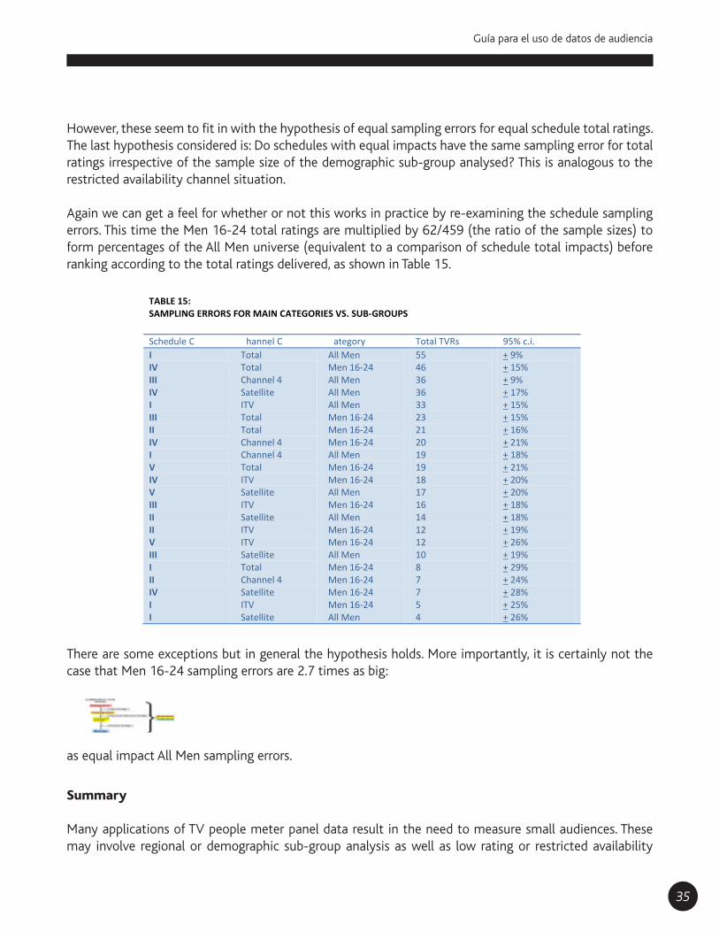
Again we can get a feel for whether or not this works in practice by re-examining the schedule sampling errors. This time the Men 16-24 total ratings are multiplied by 62/459 (the ratio of the sample sizes) to form percentages of the All Men universe (equivalent to a comparison of schedule total impacts) before ranking according to the total ratings delivered, as shown in Table 15.

There are some exceptions but in general the hypothesis holds. More importantly, it is certainly not the case that Men 16-24 sampling errors are 2.7 times as big:

as equal impact All Men sampling errors.

Summary

Many applications of TV people meter panel data result in the need to measure small audiences. These may involve regional or demographic sub-group analysis as well as low rating or restricted availability

TABLE 15: SAMPLING ERRORS FOR MAIN CATEGORIES VS. SUB-GROUPS

Schedule C hannel C ategory Total TVRs 95% c.i. I IV III IV I III II IV I V IV V III II II V III I II IV I I

Total Total Channel 4 Satellite ITV Total Total Channel 4 Channel 4 Total ITV Satellite ITV Satellite ITV ITV Satellite Total Channel 4 Satellite ITV Satellite

All Men Men 16-24 All Men All Men All Men Men 16-24 Men 16-24 Men 16-24 All Men Men 16-24 Men 16-24 All Men Men 16-24 All Men Men 16-24 Men 16-24 All Men Men 16-24 Men 16-24 Men 16-24 Men 16-24 All Men

55 46 36 36 33 23 21 20 19 19 18 17 16 14 12 12 10 8 7 7 5 4

+ 9% + 15% + 9% + 17% + 15% + 15% + 16% + 21% + 18% + 21% + 20% + 20% + 18% + 18% + 19% + 26% + 19% + 29% + 24% + 28% + 25% + 26%

36


channels. In these situations it is important to understand the sampling errors involved so that the best use of existing panel data is made.

The sampling errors associated with audience measurements of individual minutes or commercial spots are often huge. In the context of advertising schedules, any attempt at optimising the choice of individual spots is often unjustified.

However, it is well known that the total ratings for whole schedules have much lower sampling errors than the individual spots within a schedule. In fact it is broadly true that schedules with equal impacts have equal sampling errors irrespective of the size of the individual spot ratings or the sample size of the sub-groups analysed. Of course there are limiting situations in which this equality breaks down, but these would correspond to unusually heavy advertising on an individual channel.

Undoubtedly this finding will be useful in many situations. However, it cannot be allowed to generate complacency. In practice, a schedule on a low rating, restricted availability channel would never generate total impacts for a sub-group which were equal to those for a main category on a high rating, national channel.

Within the existing panels, there are measurements which provide a significantly more robust basis on which to trade advertising air time. However, in many cases there is still no substitute for increased sample size.

Alternative measurement methods for low penetration channels

Choices

A recent paper (Franz 1997) points out that small rating stations may get neglected in media planning because of their low representation on people meter panels. He suggests using independent samples collecting data, say monthly, and capable of being aggregated to large numbers of respondents in a year.

One advantage is that a large sample size made up of independent samples reduces bias which may be significant for small stations on a permanent panel. Out-of-home viewing may also be included in the measurement. He advocates normalising the viewing levels to panel levels so that data can be used com-parably (presumably separating out-of-home viewing). The use of data aggregated over time would mean that the data would be for strategic planning and the panel data would provide some tactical information.

The techniques listed by Franz for a strategic television monitor are:

personal interviews: paper or CAPI,computer aided telephone interviews,self-completion diaries.

We have a case history to report from the United Kingdom using self-completion diaries, not in the con-tinuous way suggested by Franz but as periodic snapshots.

37


Broadband Cable Audience Diary Research: A Case History

Prior to November 1997, the BARB TV people meter panel operation in the United Kingdom did not publish any audience estimates based upon the broadband cable universe because the sample sizes avai-lable were considered too small. Even now, only the five larger cable exclusive channels are itemised in the reporting system. Therefore, since January 1996, the Cable Research Group in the United Kingdom have commissioned RSMB to conduct periodic diary based studies to fulfil the broadband cable industry’s audience measurement requirements. So far, four such studies have been completed (January 1996, Sep-tember 1996, March 1997 and September 1997) and two more are due in 1998 (March and September).It must be acknowledged that a paper diary is an inferior data collection mechanism when compared to a people meter. However, the counter-argument is: what is the point of having a very precise measurement of small audiences in only a very small sample people meter panel with consequently huge sampling errors? Because it is cheaper and larger samples are therefore more affordable, a diary based study can be a more cost effective solution. Significantly the Cable TV (CATV) audience research has been formally approved by the Institute of Practitioners in Advertising (IPA) and generally accepted as providing a valid audience measurement.

The latest study (September 1997) was based upon a sample of 1300 adults and 400 children, each com-pleting a two-week quarter hour viewing diary covering all channels available in broadband cable homes. Whilst this sample size is effectively double that available from the BARB panel, we should not pretend that this completely solves the small audience measurement problem. The sampling errors for individual channels are still large. However, the value of the CATV survey is not all about increased sample size:

The diary sample is selected from an establishment survey of 2,500 households. This provides up-to-date information about the penetration and demographic profile of each broadband cable channel.Identification of the cable channels received by each diary respondent allows analysis of viewing behaviour within receivers of each channel. This is not possible within the people meter panel operation.Following the diary recording period, each respondent completes a leave behind question-naire. This is designed to collect information on usage of other media, opinions of individual channels and impressions of cable operator services, information which could not be collected from an audience measurement panel. In this way, the service is tailored to the needs of the members of the Cable Research Group.By boosting the sample it is possible to provide audience measurement data for individual cable operator areas.

A potential disadvantage of the short term diary study is its inability to measure schedule reach beyond two weeks. This is overcome with the usual probability modelling techniques which are commonly emplo-yed within radio and press research.

38


Factoring Regional Sub-Group Audiences

An approach under test in the United Kingdom for the estimation of regional sub-group audiences is that of factoring from the network panel.

The basic principle is that for a particular minute, the conversion from a main category to a sub-group rating is the same within any region as it is within the larger network panel. In algebraic terms:

where:s = sub-group rating, small area;m = main category rating, small area;S = sub-group rating, network;M = main category rating, network.By re-arranging the above formula, we can derive the basic factoring model for estimating sub-group ra-tings in small sample areas:

The model is improved by weighting the network panel to the small area panel profile before calculating the network ratings S and M.

This approach inevitably leads to results which are more stable than actual small sample based data, be-cause all the components on the right hand side of the formula are based upon larger samples. However, if the principle is not valid, then results will be biased. The purpose of the evaluation is to examine the trade-off between improved stability and potential bias.

Theoretical Reductions in Variability (Sampling Error)

The sampling error of a factored rating will be a function of the sampling errors of all three components of the factoring formula and their correlations. The mathematics of the theory are quite tortuous, but if we make some fairly well justified assumptions then the following relatively simple formula can be derived for the relationship between the sampling errors for factored and actual ratings:

where:ns = small area sub-group sample sizenm = small area main category sample size

39


Ns = network sub-group sample sizeNm = network main category sample size = expected sub-group rating = expected main category rating

The problem with this formula is that it depends upon the expected ratings levels. However, in the example in the United Kingdom where ns (small area sub-group sample size) is small compared with Nm (network main category sample size). As an example, consider Men 16-24 in London. The associated main category is All Men. First we need the relevant sample sizes. The following are effective sample sizes which reflect the weighting required to correct for geographical disproportionate sampling, demographic disproportionate sampling and other ‘accidental’ panel imbalances:

ns =London Men 16-24 effective sample size =49nm =London All Men effective sample size =322Ns =Network Men 16-24 effective sample size =421Then: In this example the sampling error is nearly halved - there is a theoretical reduction in variability of 50%.This is equivalent to a four-fold increase in the panel sample size for this sub-group.

For larger sub-groups, the reductions in sampling error are obviously not so great, as shown in Table 16.

Practical Reductions in Variability - Analysis of Variance

For applications of the TV audience measurement data which involve comparisons of sub-group ratings between regions, the sampling error approach to the assessment of variability reduction is appropriate. However, for applications which involve change over time within a single region, it must be noted that a component of the sampling error comes from the initial selection of the sample. When this sample is used on a continuous basis as a panel, the initial recruitment sampling error is equivalent to an ongoing ‘bias’. The resulting sampling errors on measurements of change over time are consequently smaller.

The analysis of variance procedure is designed to generate a practical rather than a theoretical measure-ment of the reduction in variability achieved through factoring. Published and factored ratings are calcu-

TABLE 16: THEORETICAL REDUCTIONS IN VARIABILITY

Main Category Sampling Error

Equivalent Sample Increase

Housewives with Children Women ABC1 Men 16-34 Women AB Men 16-24

29% 55% 36% 24% 14%

27% 8% 28% 28% 48%

x1.9 x1.2 x1.9 x1.9 x3.7

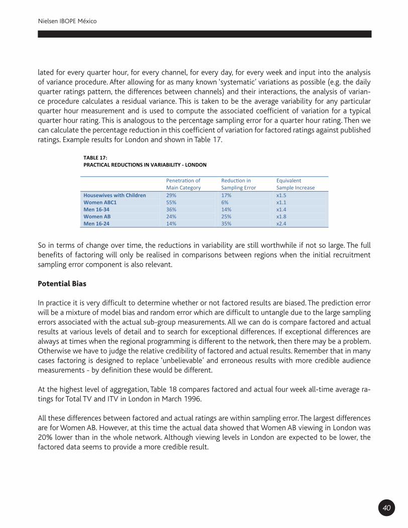
40


lated for every quarter hour, for every channel, for every day, for every week and input into the analysis of variance procedure. After allowing for as many known ‘systematic’ variations as possible (e.g. the daily quarter ratings pattern, the differences between channels) and their interactions, the analysis of varian-ce procedure calculates a residual variance. This is taken to be the average variability for any particular quarter hour measurement and is used to compute the associated coefficient of variation for a typical quarter hour rating. This is analogous to the percentage sampling error for a quarter hour rating. Then we can calculate the percentage reduction in this coefficient of variation for factored ratings against published ratings. Example results for London and shown in Table 17.

So in terms of change over time, the reductions in variability are still worthwhile if not so large. The full benefits of factoring will only be realised in comparisons between regions when the initial recruitment sampling error component is also relevant.

Potential Bias

In practice it is very difficult to determine whether or not factored results are biased. The prediction error will be a mixture of model bias and random error which are difficult to untangle due to the large sampling errors associated with the actual sub-group measurements. All we can do is compare factored and actual results at various levels of detail and to search for exceptional differences. If exceptional differences are always at times when the regional programming is different to the network, then there may be a problem. Otherwise we have to judge the relative credibility of factored and actual results. Remember that in many cases factoring is designed to replace ‘unbelievable’ and erroneous results with more credible audience measurements - by definition these would be different.

At the highest level of aggregation, Table 18 compares factored and actual four week all-time average ra-tings for Total TV and ITV in London in March 1996.

All these differences between factored and actual ratings are within sampling error. The largest differences are for Women AB. However, at this time the actual data showed that Women AB viewing in London was 20% lower than in the whole network. Although viewing levels in London are expected to be lower, the factored data seems to provide a more credible result.

TABLE 17: PRACTICAL REDUCTIONS IN VARIABILITY - LONDON

Main Category Sampling Error

Equivalent Sample Increase

Housewives with Children Women ABC1 Men 16-34 Women AB Men 16-24

29% 55% 36% 24% 14%

17% 6% 14% 25% 35%

x1.5 x1.1 x1.4 x1.8 x2.4

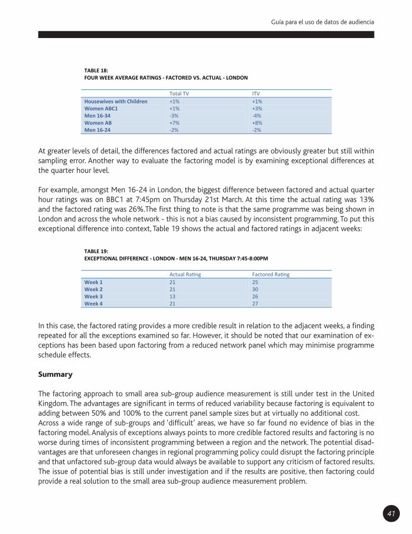
41


At greater levels of detail, the differences factored and actual ratings are obviously greater but still within sampling error. Another way to evaluate the factoring model is by examining exceptional differences at the quarter hour level.

For example, amongst Men 16-24 in London, the biggest difference between factored and actual quarter hour ratings was on BBC1 at 7:45pm on Thursday 21st March. At this time the actual rating was 13% and the factored rating was 26%.The first thing to note is that the same programme was being shown in London and across the whole network - this is not a bias caused by inconsistent programming. To put this exceptional difference into context, Table 19 shows the actual and factored ratings in adjacent weeks:

In this case, the factored rating provides a more credible result in relation to the adjacent weeks, a finding repeated for all the exceptions examined so far. However, it should be noted that our examination of ex-ceptions has been based upon factoring from a reduced network panel which may minimise programme schedule effects.

Summary

The factoring approach to small area sub-group audience measurement is still under test in the United Kingdom. The advantages are significant in terms of reduced variability because factoring is equivalent to adding between 50% and 100% to the current panel sample sizes but at virtually no additional cost.Across a wide range of sub-groups and ‘difficult’ areas, we have so far found no evidence of bias in the factoring model. Analysis of exceptions always points to more credible factored results and factoring is no worse during times of inconsistent programming between a region and the network. The potential disad-vantages are that unforeseen changes in regional programming policy could disrupt the factoring principle and that unfactored sub-group data would always be available to support any criticism of factored results.The issue of potential bias is still under investigation and if the results are positive, then factoring could provide a real solution to the small area sub-group audience measurement problem.

TABLE 19: EXCEPTIONAL DIFFERENCE - LONDON - MEN 16-24, THURSDAY 7:45-8:00PM

Week 1 Week 2 Week 3 Week 4

21 21 13 21

25 30 26 27

TABLE 18: FOUR WEEK AVERAGE RATINGS - FACTORED VS. ACTUAL - LONDON

Total TV ITV Housewives with Children Women ABC1 Men 16-34 Women AB Men 16-24

+1% +1% -3% +7% -2%

+1% +3% -4% +8% -2%

42


Summary and Conclusions

1. Mass audience commercial television channels created the need for metered panels, ultima-tely using people meters almost universally. People meters measure audience movements very precisely in terms of time, necessary for advertisement audiences but at the expense of sample size. Trading in television has been initially centred around the audiences to single spots.2. Sample size has become a severe limitation, in relation to the way in which the medium has developed, with requirements to measure ever smaller audiences. The most extreme problems are for advertisers but occur for the programming side as well.3. This paper distinguishes between different ways in which small audiences occur, considers the reliability of the data from existing systems (i.e. sampling error) and suggests possible strategies for dealing with the problem.Small audiences occur increasingly within mass audience research systems for:

arge stations at off peak times and for small sub-groups,smaller stations operating within the same universe.

4. A great deal of effort and money is wasted pursuing the single spot philosophy in situations where data are unreliable. The problems occur much higher up the scale of audience size than is always realised. The paper gives examples of sampling errors to demonstrate this.5. The solutions we suggest are:

it is worth considering whether the extra cost of increasing sample sizes might in fact save money.planning, trading and accountability need to move away from single spots to aggregated data either over weeks for single times or across whole schedules.the use of factoring for sub-group data is examined for the special case of a regionally fragmented network system.

6. Digital television will create an initially small but important growing universe. Undoubtedly this will require, initially separate, boosted people meter panels.The number and complexity of channel choice, however, will create audience fragmentation.People meter data will have to be used in an entirely different way. This will involve setting limits to the reach and share of channels. Most advertising will need to be assessed on aggre-gated data and probably schedules, extending across a range of channels. Variations in spot audiences will be meaningful in only a small number of cases. Some programming data will be useable if aggregated over time.7. Channels available to other smaller universes where meters are unaffordable, in some cases, can use alternative techniques such as paper diary panels or recall. These are ideal for evolving markets where a snapshot at a point in time provides the clearest understanding of a potential audience’s response to a channel.8. For markets which have reached a relatively stable position, surveys accumulating large samples over time may provide the basis for strategic decisions, potentially providing more reliable representation of minority interests. The problem will be the growing complexity of choice and the use of electronic programme guides which may undermine the element of awareness and recall involved in non-meter techniques.9. We believe that a crucial principle has been put forward in this paper. Sampling error is fairly

43


similar for the same number of rating points no matter whether arising from a single spot or a sche-dule.Measurement of small audiences can therefore become as reliable as for large audiences when the small audiences are combined together.10. So for the fragmented audiences of the future, research systems have to change and also the ways in which the research is used. Research users cannot go on looking at smaller audience forms by turning up the magnification of a limited microscope and seeing ever more blurred picture

References

American Research Bureau Inc. New York, ‘Arbitron replication: a study of the reliability of broadcast ra-tings’, 1974.

Boon, A.K. den ‘The reliability of television audience ratings’., in ARF/ESOMAR Worldwide Electronic and Broadcast Audience Research Symposium, 1994, Paris, France.

Franz, G. ‘How to catch small fish approaches to the measurement of small reach stations’, in: ASI 1997 European Television Symposium, 1997, Budapest, Hungary.

Read, S. and Johnson, J. ‘Audience measurement in the 21st Century’, in: ASI 1997 European Television Symposium, 1997, Budapest, Hungary

Schillmoeller, E.A. ‘Audience estimates and stability’, in: ARF/ESOMAR Worldwide Broadcast Audience Re-search Symposium, 1992, Toronto, Canada.

Twyman, T. and Wilcox, S. ‘The variability of audience measurement data and how to live with it’, in: ARF/ESOMAR Worldwide Electronic and Broadcast Audience Research Symposium, 1996, San Francisco, USA.Wilcox S. and Reeve B. ‘Statistical efficiencies in the new UK television audience measurement panels’, in: ARF/ESOMAR Worldwide Broadcast Audience Research Symposium, 1992, Toronto, Canada.

guía de uso de datos de audiencia - nielsen ibope

Documents

Transcript of guía de uso de datos de audiencia - nielsen ibope