Resumomgehrke/TeseCP.pdf · Resumo As algebras semi-De Morgan constituem uma variedade definida...
189
1 Resumo As ´ algebras semi-De Morgan constituem uma variedade definida por H. P. Sankappanavar que inclui como subvariedades a variedade K 1,1 das ´ algebras de Ockham e uma generaliza¸ c˜ ao da variedade dos reticulados distributivos pseudocomplementados tamb´ em estudada pelo mesmo autor, a variedade dos reticulados semi-pseudocomplementados. Mais tarde D. Hobby desen- volveu uma dualidade para estas ´ algebras e definiu a maior subvariedade das ´ algebras semi-De Morgan com a propriedade de extens˜ ao de congruˆ encias, a variedade C . Neste trabalho s˜ ao apresentadas desigualdades, mais simples que as en- contradas por D. Hobby, que caracterizam a variedade C e determinam-se equa¸ c˜ oes que definem as congruˆ encias principais desta variedade. Como aplica¸ c˜ ao, caracterizam-se as ´ algebras subdirectamente irredut´ ıveis de C pro- vando que para al´ em das ´ algebras subdirectamente irredut´ ıveis de K 1,1 e da variedade dos reticulados semi-pseudocomplementados s´ o existem, a menos de isomorfismo, trˆ es outras ´ algebras subdirectamente irredut´ ıveis. Explica-se de maneira detalhada um processo para obten¸ c˜ ao de duali- dades para ´ algebras com redutos reticulados distributivos que se baseia na canonicidade e na teoria de Sahlqvist e que foi obtido por M. Gehrke, H. Nagahashi e Y. Venema num artigo recente. Como aplica¸ c˜ ao determina- se uma nova dualidade para a variedade das ´ algebras semi-De Morgan e caracterizam-se os espa¸ cos duais de algumas das suas subvariedades. Estudam-se as ´ algebras semi-De Morgan que s´ o tˆ em congruˆ encias princi- pais, caracterizando-se os espa¸ cos duais dos reticulados semi-pseudocomple- mentados com esta propriedade. Generalizam-se resultados que dizem re- speito ao supremo ou ao ´ ınfimo de congruˆ encias principais, obtidos por R. Beazer para reticulados pseudocomplementados, ` a variedade dos reticulados semi-pseudocomplementados. Palavras chave: Semi-De Morgan algebras, variedade C , congruˆ encias principais, dualidade, canonicidade, Sahlqvist.
-
Upload
trinhduong -
Category
Documents
-
view
231 -
download
0
Transcript of Resumomgehrke/TeseCP.pdf · Resumo As algebras semi-De Morgan constituem uma variedade definida...

1
Resumo
As algebras semi-De Morgan constituem uma variedade definida por H. P.Sankappanavar que inclui como subvariedades a variedade K1,1 das algebrasde Ockham e uma generalizacao da variedade dos reticulados distributivospseudocomplementados tambem estudada pelo mesmo autor, a variedadedos reticulados semi-pseudocomplementados. Mais tarde D. Hobby desen-volveu uma dualidade para estas algebras e definiu a maior subvariedade dasalgebras semi-De Morgan com a propriedade de extensao de congruencias, avariedade C.
Neste trabalho sao apresentadas desigualdades, mais simples que as en-contradas por D. Hobby, que caracterizam a variedade C e determinam-seequacoes que definem as congruencias principais desta variedade. Comoaplicacao, caracterizam-se as algebras subdirectamente irredutıveis de C pro-vando que para alem das algebras subdirectamente irredutıveis de K1,1 e davariedade dos reticulados semi-pseudocomplementados so existem, a menosde isomorfismo, tres outras algebras subdirectamente irredutıveis.
Explica-se de maneira detalhada um processo para obtencao de duali-dades para algebras com redutos reticulados distributivos que se baseia nacanonicidade e na teoria de Sahlqvist e que foi obtido por M. Gehrke, H.Nagahashi e Y. Venema num artigo recente. Como aplicacao determina-se uma nova dualidade para a variedade das algebras semi-De Morgan ecaracterizam-se os espacos duais de algumas das suas subvariedades.
Estudam-se as algebras semi-De Morgan que so tem congruencias princi-pais, caracterizando-se os espacos duais dos reticulados semi-pseudocomple-mentados com esta propriedade. Generalizam-se resultados que dizem re-speito ao supremo ou ao ınfimo de congruencias principais, obtidos por R.Beazer para reticulados pseudocomplementados, a variedade dos reticuladossemi-pseudocomplementados.
Palavras chave: Semi-De Morgan algebras, variedade C, congruenciasprincipais, dualidade, canonicidade, Sahlqvist.

2
Abstract
Semi-De Morgan algebras are a subvariety, defined by H. P. Sankap-panavar, that includes as subvarieties the variety K1,1 of Ockham algebrasand a generalization of pseudocomplemented distributive lattices also studiedby the same author, the variety of demi-pseudocomplemented lattices. LaterD. Hobby developed a duality for these algebras and defined the largest sub-variety of semi-De Morgan algebras with the congruence extension property,the variety C.
In this work simpler inequalities than those found by D. Hobby to char-acterize the variety C are presented and equations defining principal con-gruences in this variety are determined. As an application, the subdirectlyirreducible algebras of C are characterized and it is proved that apart fromthe subdirectly irreducible algebras of K1,1 and of the variety of demi-pseudo-complemented algebras there are, up to isomorphism, just three other sub-directly irreducible algebras.
It is spelled out a process of obtaining dualities for distributive lattice-ordered algebras based on canonicity and on the Sahlqvist theory that wasdeveloped by M. Gehrke, H. Nagahashi and Y. Venema in a recent article.As an application it is determined a new duality for the variety of semi-DeMorgan algebras and the dual spaces of some of its subvarieties are charac-terized.
Semi-De Morgan algebras having only principal congruences are alsostudied and the dual spaces of demi-pseudocomplemented lattices with thisproperty are characterized. Results on the principal join property and theprincipal intersection property that were obtained by R. Beazer for pseu-docomplemented distributive lattices are generalized to the variety of demi-pseudocomplemented lattices.
Keywords: Semi-De Morgan algebras, variety C, principal congruences,duality, canonicity, Sahlqvist.

3
Acknowledgements
First I want to thank my advisor, Professor Raquel Santos, for her teach-ings, her patience and her continuous support throughout this research andmy co-advisor, Professor Mai Gehrke, for her advice and encouragement.
Many thanks to all the people at Departamento de Matematica, Facul-dade de Ciencias and at Centro de Algebra da Universidade de Lisboa whohave helped me with their suggestions and their interest in my work. I par-ticularly want to thank Professor Luıs Sequeira for all his patience in solvingmy problems with Latex.
Finally I want to express my gratitude to the institutions below for theirfinancial support,
-Departamento de Matematica da Faculdade de Ciencias da Universidadede Lisboa
-Centro de Algebra da Universidade de Lisboa-Fundacao para a Ciencia e Tecnologia-Fundacao Luso-Americana.

4
Contents
1 Preliminaries 23
1.1 Ordered Structures . . . . . . . . . . . . . . . . . . . . . . . . 23
1.2 Universal Algebra . . . . . . . . . . . . . . . . . . . . . . . . . 24
1.2.1 Classes of algebras of the same type . . . . . . . . . . . 25
1.3 Lattices . . . . . . . . . . . . . . . . . . . . . . . . . . . . . . 25
1.3.1 Pseudocomplemented distributive lattices . . . . . . . . 28
1.3.2 Ockham algebras . . . . . . . . . . . . . . . . . . . . . 28
1.4 Semi-De Morgan algebras . . . . . . . . . . . . . . . . . . . . 29
2 The variety C 33
2.1 The variety C of semi-De Morgan algebras . . . . . . . . . . . 33
2.2 Principal congruences in the variety C . . . . . . . . . . . . . . 40
2.3 Subdirectly irreducibles in variety C. . . . . . . . . . . . . . . 49
2.4 Equational Bases for some Subvarieties. . . . . . . . . . . . . 58
3 Duality 61
3.1 Canonical extension and canonicity . . . . . . . . . . . . . . . 61
3.1.1 Canonical extensions of Distributive Lattices . . . . . . 61
3.1.2 Canonical extensions of Distributive Algebras . . . . . 68
3.1.3 Sahlqvist inequalities and canonicity . . . . . . . . . . 70
3.2 Discrete Duality . . . . . . . . . . . . . . . . . . . . . . . . . . 73
3.2.1 Basic technical ingredients . . . . . . . . . . . . . . . 73
3.2.2 A duality for UQA+s . . . . . . . . . . . . . . . . . . . 86
3.3 Discrete duality for Canonical Extensions . . . . . . . . . . . . 97
3.4 Basic Topological duality . . . . . . . . . . . . . . . . . . . . . 100
3.4.1 Bounded Distributive Lattices . . . . . . . . . . . . . . 100
3.4.2 Distributive Algebras . . . . . . . . . . . . . . . . . . . 110
5

6 CONTENTS
4 A duality for SDMAs 1214.1 Canonicity . . . . . . . . . . . . . . . . . . . . . . . . . . . . . 121
4.1.1 Discrete Correspondence . . . . . . . . . . . . . . . . . 1244.2 Correspondence for canonical extensions . . . . . . . . . . . . 133
4.2.1 Topological duality for SDMAs . . . . . . . . . . . . . 1404.3 The dual spaces of some subvarieties of SDMA . . . . . . . . 147
5 Some properties of congruences 1595.1 Congruences and duality in DL . . . . . . . . . . . . . . . . . 1595.2 Congruences and duality in SDMA . . . . . . . . . . . . . . . 1635.3 SDMAs having only principal congruences . . . . . . . . . . . 1665.4 The principal join property . . . . . . . . . . . . . . . . . . . . 1715.5 The Principal Intersection Property . . . . . . . . . . . . . . . 177
A 179

Introduction
Many varieties of algebras consisting of bounded distributive lattices withadditional unary operations have been studied as algebraic models for certainlogics. They include well known examples, such as Ockham, MS, De Morgan,Stone, and Boolean algebras as well as pseudo-complemented lattices.
For some of these varieties there are several similar properties so it isnatural to look for generalizations where these properties still hold.
This is the case of De Morgan algebras (DMAs) and distributive pseudo-complemented lattices (also called p-lattices) where the presence of commonaspects made Sankappanavar consider in [38] the more general variety ofsemi-De Morgan algebras (SDMAs).
Sankappanavar continued the investigation of SDMAs in [39] and [40],where he concentrated on the subvariety of demi-pseudocomplemented lat-tices (also called demi-p-lattices, (DMPLs)) and on almost pseudocomple-mented lattices (also called almost p-lattices, (APLs)), a subvariety of demi-p-lattices. These are generalizations of p-lattices and they don’t include thevariety of De Morgan algebras.
Using algebraic techniques, Sankappanavar characterized in [38] some im-portant subvarieties of SDMAs and proved that certain elements of a semi-De Morgan algebra form a De Morgan algebra, extending the well knowntheorem for p-lattices due to Glivenko.
When he restricted his study to DMPL in [39] and [40], Sankappanavardetermined equations defining principal congruences and, as an application,characterized the subdirectly irreducible algebras. He also determined thelattice of subvarieties of DMPL.
Since we started this study, our main goal has been the investigation of thecorresponding results for the variety SDMA. We studied in [26] the latticeof congruences of subdirectly irreducible algebras in SDMA. However, ourattempt to go further using algebraic methods was not fruitful since SDMA
7

8 CONTENTS
does not have the congruence extension property (CEP ).
Using topological methods, D. Hobby developed in [25] a duality forSDMA based on the Priestley duality for distributive lattices. As an ap-plication, he characterized the dual spaces of subdirectly irreducible semi-DeMorgan algebras and he determined the largest subvariety of SDMA withthe congruence extension property which he called the variety C.
Hobby’s duality is described by himself as ”tractable enough to be useful”however with conditions that ”seem inelegant” so, he suggests, as Problem 1of his article, a duality for SDMAs ”more nicely stated”.
Since the variety SDMA does not have the congruence extension prop-erty, Hobby observed that perhaps it is too large to be useful as a com-mon generalization of DMAs and p-lattices. Therefore C turns out to bevery interesting because it has CEP and it contains all the previously stud-ied subvarieties of SDMA, namely the subvariety K1,1 of Ockham algebras(consequently DMA) and DMPL.
However the two inequalities (α and β) that characterize C as a subvarietyof SDMA in [25] are too complicated to make the study of C very tempting.
In fact Problem 2 in [25] is to find ”nicer axioms for C”.
We solved this problem algebraically determining a new inequality (γ)such that C can be characterized by γ and β.
We determined the equations defining principal congruences in C and wecharacterized the subdirectly irreducible algebras of this variety.
Blyth and Varlet characterized in [9] the distributive lattices, the Stone,the De Morgan and the Heyting algebras that have only principal congru-ences. In [6], Beazer solved the same problem for p-lattices. It was naturalto ask whether their results could be extended. Using algebraic techniques,analogous to those used by Beazer in [5] and [6], we proved, in [27], that thesemi-De Morgan algebras with the referred property are finite so that, whenapplying Hobby’s duality, we could drop the topology because, in this case,it is the discrete one. Using this method we generalized to demi-p-latticesresults obtained by Beazer in [5] and [6].
We continued the study of principal congruences, concentrating on alge-bras that have the principal join property (PJP ), i.e. those algebras suchthat the join of any two principal congruences is a principal congruence.Beazer characterizes p-lattices with this property in [5]. In [12], I. Chadacalls these algebras congruence principal and, in [13] he studies algebraswhose principal congruences form a sublattice of their congruence lattice. In

CONTENTS 9
[29] we apply Hobby’s duality to the study of this property in what concernsdemi-p-lattices and we prove, generalizing a result by Beazer [5], that in thisvariety those algebras having the principal join property have the principalintersection property. This solves, for demi-p-lattices, problem 6 proposedby Hobby in [25].
The difficulties we found when dealing with Hobby’s duality motivatedus to try to find a simpler alternative for this duality.
While searching for a duality for SDMA we decided to follow the sug-gestions of Professor M. Gehrke and to apply Canonicity and the SahlqvistTheory to this study.
Canonical extensions provide a complete lattice theoretic view of topo-logical duality for various types of lattice and even poset-ordered algebras[18, 20, 22]. They were first developed by Jonsson and Tarski for Boolean al-gebras with additional operations that preserve join in each coordinate. Morerecently, generalizations and stronger results about preservation of identitiesunder canonical extensions have been obtained by M. Gehrke and B. Jonssonand others. The paper [21] is particularly useful for our purposes. In thispaper M. Gehrke, H. Nagahashi and Y. Venema use the modern theory ofcanonical extensions to generalize powerful results from modal logic aboutpreservation of identities and relational correspondents for these equations.The results in that paper are cast as a generalization of Sahlqvist theory forcertain generalized modal logics based on distributive lattices. However, asthe authors also comment, these results may also be seen as a general theoryfor manufacturing topological dualities for the distributive lattice-ordered al-gebras corresponding to the logics they treat. In this work we will spell outthe parts of this process and apply it in the case of the variety of semi-DeMorgan algebras and various subvarieties of this variety.
In this work, to avoid confusion with De Morgan algebras, we denoteby unary quasi-operators algebras (UQAs) the distributive modal algebrasconsidered in [21] by M.Gehrke, H. Nagahashi and Y. Venema, since theunary operations 3,2,B and C are called unary quasi-operators in [22].
We follow [21] to determine a duality between the canonical extensionsof these algebras and the corresponding ordered relational structures. Weobtain the dual spaces of UQAs by defining a topology in these orderedspaces.
It is clear that these results also apply to algebras that are the reducts ofUQAs so we consider distributive algebras with the unary operations 2 and

10 CONTENTS
B. In this setting we can characterize the variety SDMA introducing addi-tional inequalities satisfied by the unary operations. These inequalities are,according to the definition in [21], Sahlqvist inequalities and hence canonical.
M.Gehrke, H. Nagahashi and Y. Venema proved in [21] that every Sahlqvistmodal sequent corresponds to a formula in the dual frame. It is clear thatthe same happens to Sahlqvist inequalities and conditions in the dual space.We applied this result to compute quite easily the formulas corresponding toSahlqvist inequalities.
Since SDMA, as well as important subvarieties such as C, DMPL, K1,1,can be defined by Sahlqvist inequalities, we established a duality for SDMAand we characterized the dual spaces of the referred subvarieties.
The first chapter of this thesis contains definitions and results that willbe needed later.
We assume familiarity with basic concepts of universal algebra and latticetheory.
In section 1.4 we present the definition of semi-De Morgan algebras andimportant properties of these algebras. For a more detailed exposition see[38], [39] and [40].
In chapter 2, we solve Problem 2 from [25]. We determine algebraicallyan inequality (γ) such that inequalities γ and β characterize C as a subvarietyof SDMA. In Sections 2 and 3 we include results that were obtained in [28]:We characterize the principal congruences on C, extending the correspond-ing characterization for demi-p-lattices, due to Sankappanavar [39], and forthe variety K1,1 due to J. Berman [8] and to M. Ramalho and M. Sequeira[33]. It is shown that C has equationally definable principal congruences,a result which strengthens Hobby’s result that this variety has congruenceextension property. We also determine the subdirectly irreducible algebrasof the variety C. The subdirectly irreducible demi-p-lattices were character-ized by Sankappanavar in [39] and the subdirectly irreducible algebras of thevariety K1,1 were identified in [37] and also in [5]. We use these results andthe characterization of principal congruences to prove that apart from thesubdirectly irreducible algebras of the varieties of demi-p-lattices and K1,1
there are, up to isomorphisms, three more subdirectly irreducible algebras inC. We consider the set consisting of the isomorphism classes of finite subdi-rectly irreducible algebras of the variety C and we present the Hasse diagramof this poset. Using a theorem of B. Davey [16], we prove that the lattice ofsubvarieties of C is isomorphic to the lattice of order-ideals of this poset. In

CONTENTS 11
Section 4 we give defining identities for some subvarieties of C.Chapters 3 and 4 concern the study of duality based on the theory of
canonical extensions. This is a general program that will be illustrated here.
In chapter 3 we will give some results on canonical extensions for dis-tributive lattices (DL ). As our results may be seen mainly as an applicationof the results in [21], we will refer to this paper and we will try to conform tothe notation and nomenclature used there. For further references on canon-ical extensions we will refer to the most recent and comprehensive paper byGehrke and Jonsson [20] even for results first proved earlier.
In section 3.2 we consider the class of Perfect Distributive Lattices (DL+).These are completely distributive lattices that are join generated by the setof completely join irreducible elements and they include the class of canonicalextensions of distributive lattices.
Following [21], we establish a duality between DL+ and posets: Givena lattice in DL+ the completely join irreducible elements form a poset and,given a poset, the downsets form a lattice in DL+. In this way it is obtaineda generalization of Birkhoff’s duality for finite distributive lattices.
At the objects level this was already done by G. Raney [34], V. Balachan-dran [3] and P. Dwinger [4].
When we expand perfect distributive lattices with additional unary op-erations (3,2,B and C), we obtain the class of algebras that we denote byUQA+ and we explain how in [21] the authors determine the correspondingduality endowing the dual posets with binary relations.
The fact that a lattice in DL is a lattice in DL+ has important conse-quences that we discuss in section 3.3.
The duality for the category DL+ is applied in section 3.4 to define aduality for bounded distributive lattices (DL). This is done by introducinga topology in the dual poset of completely join irreducible elements of thecanonical extensions of lattices in DL. In the end what we obtain is a versionof Priestley duality.
This kind of approach of Priestley duality for distributive lattices has,among others, the advantage of defining the dual space as a subset of thecanonical extension of the distributive lattice. Besides, when dealing withfinite distributive lattices, we fall directly in Birkhoff’s duality.
To determine a duality for UQA, we have just to find how the topologyin the Priestley space (dual of the underlying distributive lattice) interactswith the additional binary relations in the dual space of UQA+. This is done

12 CONTENTS
in detail for the join preserving operation and then generalized to the otherunary operations using the appropriate order duals of the distributive lattice.
Using Priestley duality, R. Goldblatt developed in [23], a representationfor distributive lattices with operators that are meet or join preserving. Later,in [41], V. Sofronie-Stokermans generalized this duality to meet or join re-versing operators. Though we work in a different setting their results werevery useful.
As an application of this duality, we develop in chapter 4 a duality forSDMA. We start by considering, in section 4.1, a class of distributive latticesextended with the unary operations B and 2. This is a reduct of UQA wherewe define the variety SDMA by a set of inequalities that are satisfied by theunary operations.
These inequalities are Sahlqvist so, applying results established by M.Gehrke, H. Nagahashi and Y. Venema in [21], we conclude that they arecanonical and hence SDMA is a canonical variety. Therefore the canonicalextension of an algebra in SDMA is still in SDMA. In fact it is in a classof algebras that we call SDMA+ which is the intersection of UQA+ andSDMA. Since in the previous chapter we have already established a dualityfor UQA+, we apply this duality and the Sahlqvist theory in [21] to computethe formulas corresponding to the Sahlqvist inequalities in the dual space.This way we characterize the binary relations that correspond to B and 2 inthe dual structure of SDMA+. But these two relations are not independentso we can define morphisms between dual structures of SDMA+ by lessconditions than in UQA+.
The minimal elements in the codomain of one of the binary relations arethe maximal elements in the codomain of the other so that we can define anew binary relation having as codomain this set of elements. In section 4.2,we consider the case of algebras in SDMA+ that are canonical extensions ofalgebras in SDMA. Then, this new binary relation is particularly interestingbecause we can obtain a much simpler duality for SDMA+.
To capture a duality for SDMA we have, as for UQA, to consider thetopology in the dual space and to determine how the new binary relationbehaves regarding this topology. This way we finish by establishing a fullduality for SDMA.
As an application of this duality, we characterize, in section 4.3, thedual spaces of some important subvarieties of SDMA that are defined bySahlqvist inequalities and compare the duality we have established with the

CONTENTS 13
correspondent known dualities.
In chapter 5, applying the duality for SDMAs presented in the previouschapter, we study the properties of principal congruences in SDMA consid-ered in [27] and [29]. Generalizing results obtained by R. Beazer in [5] and[6], we show that SDMAs having only principal congruences are finite. Next,using duality, we show how demi-p-lattices and almost p-lattices having onlyprincipal congruences can be described.
We also characterize those demi-p-lattices having the principal join prop-erty extending the corresponding results obtained by Beazer in [5]. We alsoprove that those algebras in DMPL having the principal join property havethe principal intersection property.
We observe that some of the results presented in chapters 2 and 5 werejoint work with Professor Raquel Santos.
14 CONTENTS

Introducao
Muitas variedades de algebras tais como as algebras de Ockham, as algebrasMS, de De Morgan, de Stone e de Boole bem como os reticulados pseudocom-plementados sao exemplos bem conhecidos de algebras tendo como redutoum reticulado distributivo limitado com uma operacao unaria adicional.
Nalgumas destas variedades, que tem sido estudadas como modelos alge-bricos de certas logicas, ha propriedades que sao semelhantes pelo que enatural procurar generalizacoes em que estas propriedades se continuam averificar.
E este o caso das algebras de De Morgan (DMAs) e dos reticuladosdistributivos pseudocomplementados (tambem designados por reticulados-p)onde a presenca de aspectos comuns levou Sankappanavar a considerar em[38] a variedade mais geral das algebras semi-De Morgan (SDMAs).
Em [39] e em [40], Sankappanavar continuou a investigacao sobre SDMAsconcentrando o seu estudo nas subvariedades dos reticulados semi-pseudo-complementados (tambem designados por reticulados semi-p, (DMPLs)) edos reticulados quase-pseudocomplementados (tambem designados por retic-ulados quase-p, (APLs)). Ambas sao generalizacoes dos reticulados-p quenao incluem a variedade das algebras de De Morgan.
Usando tecnicas algebricas, Sankappanavar caracterizou em [38] algumassubvariedades importantes de SDMA e provou que determinados elemen-tos de uma algebra semi-De Morgan formam uma algebra de De Morgan,extendendo assim o bem conhecido teorema de Glivenko para reticulados-p.
Quando restringiu o seu estudo a DMPL em [39] e em [40], Sankap-panavar determinou equacoes que definem as congruencias principais e, comoaplicacao, caracterizou as algebras subdirectamente irredutıveis desta var-iedade. Determinou, tambem, o reticulado das subvariedades de DMPL.
Quando iniciamos este estudo, o nosso principal objectivo era a inves-
15

16 CONTENTS
tigacao dos resultados correspondentes para a variedade SDMA. Estudamosem [26] o reticulado das congruencias das algebras subdirectamente irre-dutıveis de SDMA. Contudo, as tentativas para ir mais alem usando metodosalgebricos foram infrutıferas porque SDMA nao tem a propriedade de ex-tensao de congruencias (CEP ).
Usando metodos topologicos, D. Hobby desenvolveu em [25] uma duali-dade para SDMA baseada na dualidade de Priestley para reticulados dis-tributivos. Como aplicacao desta dualidade, caracterizou os espacos duais dasalgebras semi-De Morgan subdirectamente irredutıveis e determinou a maiorsubvariedade de SDMA com a propriedade de extensao de congruencias quedesignou por variedade C.
A dualidade de Hobby e descrita por ele proprio como ”suficientementetratavel para ser util” contudo com condicoes que ”parecem deselegantes”.Em consequencia, como Problema 1 do seu artigo, Hobby sugere a deter-minacao de uma nova dualidade para SDMAs.
Como a variedade SDMA nao tem a propriedade de extensao de con-gruencias, Hobby observou que talvez seja grande demais para ser util comogeneralizacao comum das DMAs e dos reticulados-p. A variedade C torna-seportanto muito interessante porque tem CEP e contem todas as subvar-iedades de SDMA previamente estudadas, nomeadamente a subvariedadeK1,1 das algebras de Ockham (logo DMA) e DMPL. Contudo as desigual-dades α e β que caracterizam C como subvariedade de SDMA em [25] saoexcessivamente complicadas para tornar o estudo de C tentador.
De facto o Problema 2 de [25] e a determinacao de axiomas mais elegantespara C.
Resolvemos este problema algebricamente determinando uma nova de-sigualdade (γ) tal que C e caracterizavel por γ e β.
Determinamos tambem equacoes que definem as congruencias principaisem C e caracterizamos as algebras subdirectamente irredutıveis desta var-iedade.
Os reticulados distributivos, as algebras de Stone, de De Morgan e deHeyting que so tem congruencias principais foram caracterizados por Blythe Varlet em [9]. Beazer resolveu o mesmo problema para reticulados-p em[6]. Pos-se assim naturalmente a questao de saber se estes resultados saogeneralizaveis. Aplicando tecnicas algebricas analogas as usadas por Beazerem [5] e em [6], provamos, em [27], que as algebras semi-De Morgan que sotem congruencias principais sao finitas logo, ao aplicar a dualidade de Hobby,

CONTENTS 17
pudemos ignorar a topologia uma vez que neste caso e a topologia discreta.Usando este metodo generalizamos a reticulados semi-p resultados obtidospor Beazer em [5] e em [6].
Continuando o estudo das congruencias principais, consideramos as alge-bras tais que o supremo de quaisquer duas congruencias principais e uma con-gruencia principal (algebras com a propriedade PJP ). Beazer caracteriza osreticulados-p com esta propriedade em [5]. I. Chada [12], chama congruentesprincipais a estas algebras e, em [13], estuda algebras cujas congruenciasprincipais formam um subreticulado do reticulado das congruencias. Em[29], aplicamos a dualidade de Hobby para estudar esta propriedade nosreticulados semi-p e provamos, generalizando um resultado de Beazer [5],que nesta variedade as algebras que tem a propriedade PJP tem tambema propriedade de a interseccao de quaisquer duas congruencias principaisser uma congruencia principal (propriedade PIP ). Resolvemos assim parareticulados semi-p o Problema 6 proposto por Hobby em [25].
As dificuldades encontradas ao aplicar a dualidade de Hobby motivaramo estudo de uma alternativa mais simples a esta dualidade.
Ao procurar uma dualidade para SDMA decidimos aceitar a sugestao daProfessora M. Gehrke e aplicar a Canonicidade e a Teoria de Sahlqvist a esteestudo.
As extensoes canonicas foram desenvolvidas inicialmente por Jonsson eTarski para algebras Booleanas com operacoes adicionais que preservam osupremo em cada coordenada. Mais recentemente, generalizacoes e resulta-dos mais fortes sobre a preservacao de identidades em extensoes canonicasforam obtidos por M. Gehrke e B. Jonsson e por outros. O artigo [21] eparticularmente util para os nossos objectivos. Neste artigo M. Gehrke, H.Nagahashi e Y. Venema usam a moderna teoria das extensoes canonicaspara generalizar resultados poderosos da logica modal sobre a preservacaode identidades e as condicoes relacionais que lhes correspondem. Os resul-tados desse artigo sao apresentados como uma generalizacao da teoria deSahlqvist para certas logicas modais generalizadas baseadas em reticuladosdistributivos. Contudo, como os autores tambem comentam, estes resultadospodem ser vistos como uma teoria geral para obter dualidades topologicaspara as algebras com redutos reticulados distributivos correspondentes aslogicas consideradas. Neste trabalho explicamos detalhadamente as partesdeste processo e aplicamo-lo ao caso da variedade das algebras semi-De Mor-gan e de algumas das suas subvariedades.
18 CONTENTS
Para evitar confusao com as algebras de De Morgan (DMAs), ao longodeste trabalho chamamos algebras de quase-operadores unarios (UQAs) asalgebras modais distributivas consideradas em [21] por M.Gehrke, H. Naga-hashi e Y. Venema, uma vez que as operacoes unarias 3,2,B and C saodesignadas por quase-operadores unarios em [22].
Seguimos [21] para determinar uma dualidade entre as extensoes canonicasdestas algebras e certas estruturas relacionais ordenadas. Obtemos os espacosduais das UQAs definindo uma topologia nestas estruturas relacionais orde-nadas.
Como estes resultados tambem se aplicam a algebras que sao redutos deUQAs, podemos considerar algebras distributivas com as operacoes unarias 2
e B. Neste contexto a variedade SDMA pode ser caracterizada por meio dedesigualdades adicionais nas operacoes unarias. Estas desigualdades sao, deacordo com a definicao dada em [21], desigualdades de Sahlqvist e portantosao canonicas.
Foi provado em [21] que toda a sequencia modal de Sahlqvist correspondea uma formula na estrutura dual. Como o mesmo acontece com desigual-dades de Sahlqvist e condicoes no espaco dual, aplicamos este resultado paradeduzir, com bastante facilidade, as formulas que correspondem as desigual-dades de Sahlqvist.
Tanto SDMA como subvariedades importantes tais como C, DMPL eK1,1 podem ser definidas por desigualdades de Sahlqvist. Estabelecemos as-sim uma dualidade para SDMA e caracterizamos o espaco dual das referidassubvariedades.
O primeiro capıtulo desta tese contem definicoes e resultados que seraonecessarios posteriormente.
Pressupomos familiariedade com conceitos basicos de Algebra Universale da Teoria dos Reticulados.
Na seccao 1.4 apresentamos a definicao de algebra semi-De Morgan ealgumas propriedades importantes destas algebras. Para informacao maisdetalhada sugerimos [38], [39] and [40].
No Capıtulo 2, resolvemos o Problema 2 de [25]. Determinamos algebri-camente uma desigualdade (γ) tal que as desigualdades γ and β caracterizamC como subvariedade de SDMA.
Nas Seccoes 2 e 3 incluimos resultados que foram obtidos em [28]: Car-acterizamos as congruencias principais em C, generalizando a caracterizacaocorrespondente para reticulados semi-p obtida por Sankappanavar [39], e

CONTENTS 19
para a variedade K1,1 obtida por J. Berman [8] e por M. Ramalho e M. Se-queira [33]. Mostra-se que C tem congruencias principais equacionalmentedefinıveis, um resultado que confirma que esta variedade tem a propriedadede extensao de congruencias como Hobby provou. Determinamos tambem asalgebras subdirectamente irredutıveis da variedade C. Os reticulados semi-p subdirectamente irredutıveis foram caracterizados por Sankappanavar em[39] e as algebras subdirectamente irredutıveis da variedade K1,1 foram iden-tificadas em [37] e tambem em [5]. Usamos estes resultados e a caracterizacaodas congruencias principais para provar que para alem das algebras subdi-rectamente irredutıveis das variedades dos reticulados semi-p e de K1,1 ha,a menos de isomorfismo, mais tres algebras subdirectamente irredutıveis emC. Apresentamos o diagrama de Hasse do conjunto parcialmente ordenadodas classes de isomorfismo das algebras finitas subdirectamente irredutıveisda variedade C. Usando um teorema de B. Davey [16], provamos que o retic-ulado das subvariedades de C e isomorfo ao reticulado dos semi-ideais desteconjunto.
Na seccao 2.4 apresentamos identidades que caracterizam algumas sub-variedades de C.
Os capıtulos 3 e 4 incluem o estudo da dualidade baseada na teoria dasextensoes canonicas.
No capıtulo 3 damos alguns resultados sobre extensoes canonicas de retic-ulados distributivos (DL ). Como os nossos resultados podem ser consider-ados principalmente como uma aplicacao dos resultados obtidos em [21],fazemos referencia a este artigo e usamos notacao e nomenclatura adaptadaa que e aı usada. Para outras referencias relativas a extensoes canonicasrecorremos ao artigo mais recente e mais abrangente de Gehrke e Jonsson[20] mesmo para resultados ja provados anteriormente.
Na seccao 3.2 consideramos a classe dos Reticulados Distributivos Per-feitos (DL+). Sao reticulados completamente distributivos que sao sup-gerados pelo conjunto dos elementos completamente sup-irredutıveis e in-cluem a classe das extensoes canonicas dos reticulados distributivos.
De acordo com [21], estabelecemos uma dualidade entre DL+ e conjuntosparcialmente ordenados: Dado um reticulado em DL+, os elementos comple-tamente sup-irredutıveis constituem um conjunto parcialmente ordenado e,dado um conjunto parcialmente ordenado, os semi-ideais formam um retic-ulado em DL+. Deste modo obtem-se uma generalizacao da dualidade deBirkhoff para reticulados distributivos finitos.

20 CONTENTS
Isto ja havia sido feito, ao nıvel dos objectos, por G. Raney [34], V.Balachandran [3] e P. Dwinger [4].
Quando se expandem reticulados distributivos perfeitos com operacoesunarias adicionais (3,2,B and C), obtem-se a classe de algebras que des-ignamos por UQA+. Explicamos como em [21] M. Gehrke, H. Nagahashi eY. Venema determinam a dualidade correspondente munindo os conjuntosparcialmente ordenados duais com relacoes binarias.
O facto de um reticulado em DL ser um reticulado em DL+ tem con-sequencias importantes que discutimos na seccao 3.3.
A dualidade para a categoria DL+ e aplicada na seccao 3.4 para definiruma dualidade para reticulados distributivos limitados (DL). Para o fazer in-troduzimos uma topologia no conjunto parcialmente ordenado dos elementoscompletamente sup-irredutıveis, dual da extensao canonica dum reticuladode DL. No fim o que se obtem e uma versao da dualidade de Priestley.
Este tipo de abordagem da dualidade de Priestley para reticulados dis-tributivos tem, entre outras, a vantagem de definir o espaco dual como umsubconjunto da extensao canonica do reticulado distributivo e de, quando seconsideram reticulados distributivos finitos, se ir cair directamente na duali-dade de Birkhoff.
Para determinar uma dualidade para UQA, basta estudar o modo como atopologia no espaco de Priestley (dual do reticulado distributivo subjacente)interage com as relacoes binarias adicionais do espaco dual de UQA+.
Este estudo e feito em detalhe para a operacao que preserva o supremoe generalizado depois as outras operacoes unarias usando os duais de ordemapropriados.
Usando a dualidade de Priestley, R. Goldblatt desenvolveu em [23] umarepresentacao para reticulados distributivos com operadores que preservamo supremo ou o ınfimo. Mais tarde, em [41], V. Sofronie-Stokermans gen-eralizou esta dualidade a operadores que invertem o supremo ou o ınfimo.Apesar de trabalharmos num contexto diferente os resultados obtidos porestes autores foram-nos muito uteis.
Como aplicacao da dualidade que obtivemos, desenvolvemos no capıtulo 4uma dualidade para SDMA. Comecamos por considerar, na seccao 4.1, umaclasse de reticulados distributivos com as operacoes unarias B e 2. Trata-sede um reduto de UQA onde definimos a variedade SDMA por um conjuntode desigualdades que tem que ser satisfeitas pelas operacoes unarias. Estassao desigualdades de Sahlqvist e portanto, aplicando resultados estabeleci-

CONTENTS 21
dos por M. Gehrke, H. Nagahashi e Y. Venema em [21], concluımos que saocanonicas logo SDMA e uma variedade canonica. Consequentemente a ex-tensao canonica de uma algebra em SDMA esta ainda em SDMA. De factoesta numa classe de algebras a que chamamos SDMA+ e que e a interseccaode UQA+ e SDMA. Como no capıtulo anterior ja tinhamos estabelecidouma dualidade para UQA+, aplicamos esta dualidade e a teoria de Sahlqvistde [21] para calcular as formulas que correspondem, no espaco dual, as de-sigualdades. Deste modo caracterizamos as relacoes binarias que correspon-dem a B e a 2 na estrutura dual de SDMA+. Como estas duas relacoesnao sao independentes podemos definir os morfismos entre estruturas duaisde SDMA+ por menos condicoes que em UQA+.
Os elementos minimais do codomınio de uma das relacoes binarias sao oselementos maximais do codomınio da outra de modo que e possıvel definiruma nova relacao binaria tendo como codomınio este conjunto de elementos.Na seccao 4.2, consideramos o caso de algebras de SDMA+ que sao extensoescanonicas de algebras de SDMA. Neste caso esta nova relacao binaria eparticularmente interressante porque permite obter uma dualidade muitomais simples para SDMA+.
Tal como em UQA, para obter uma dualidade para SDMA consideramosa topologia do espaco dual e determinamos o modo como a nova relacaobinaria se comporta relativamente a esta topologia.
Como aplicacao desta dualidade, caracterizamos, na seccao 4.3, os espacosduais de algumas subvariedades importantes de SDMA que sao definidas pordesigualdades de Sahlqvist e comparamos a dualidade que estabelecemos comas correspondentes dualidades ja conhecidas.
No capıtulo 5, com a dualidade para SDMAs que apresentamos no capıtuloanterior, estudamos as propriedades das congruencias principais em SDMAconsideradas em [27] e [29]. Assim, generalizando resultados obtidos porBeazer em [5] e em [6], mostramos que SDMAs que so tem congruenciasprincipais sao finitas e esclarecemos como podem ser descritos os reticuladossemi-p e quase-p que so tem congruencias principais.
Caracterizamos, tambem, os reticulados semi-p com a propriedade PJPfazendo uma extensao dos resultados correspondentes obtidos por Beazer em[5]. Provamos que as algebras de DMPL com a propriedade PJP tem aindaa propriedade PIP .
De notar que parte dos resultados referidos nos capıtulos 2 e 5 foram umtrabalho conjunto com a Professora Raquel Santos.

22 CONTENTS
Chapter 1
Preliminaries
We assume that the basic notions of Universal Algebra and Lattice Theoryare known. Anyway we list here some definitions and results that will bedirectly related with our study.
For more details concerning these subjects, we refer the reader to R.Balbes and P. Dwinger [4], S. Burris and H. P. Sankappanavar [11], B. A.Davey and H. A. Priestley [17].
1.1 Ordered Structures
Let (X,≤) be a partially ordered set (poset) and let x, y ∈ X. We say thatx is covered by y and we write x � y (or y � x) if x < y and there is noelement z ∈ X for which x < z < y.
A subset S of a poset X is called convex if x, y ∈ S and z ∈ X andx ≤ z ≤ y imply that z ∈ S.
If X is a poset then we say that X has height less than or equal tok ∈ N and we write h(X) ≤ k if every chain in X has at most k+ 1 elements.
Notice that a partially ordered set X is such that h(X) ≤ 1 if and onlyif all its subsets are convex.
Let (X,≤) be a poset and let S ⊆ X. We say that S is a downset (or anorder ideal) if, whenever x ∈ S, y ∈ X and y ≤ x, we have y ∈ S. Dually,S is an upset (or an order filter) if, whenever x ∈ S, y ∈ X and x ≤ y, wehave y ∈ S.
23

24 CHAPTER 1. PRELIMINARIES
Given an arbitrary subset S ⊆ X, we define
↓ S = {y ∈ X : ∃x ∈ S y ≤ x} and ↑ S = {y ∈ X : ∃x ∈ S y ≥ x}.
When S = {x} with x ∈ X we denote ↓ S and ↑ S by ↓ x and ↑ x,respectively.
The family of all down-sets of X is denoted by D(X).
Let X be a poset. A non-empty subset S ⊆ X is said to be up-directedif, for any x, y ∈ S, there exists an upper bound z ∈ S. Dually S is down-directed if, for any x, y ∈ S, there exists a lower bound z ∈ S.
A poset X is defined to be up-complete if every up-directed subset has ajoin in X. If every down-directed subset has a meet in X we say that X isdown-complete.
Every lattice L can be regarded as an ordered set (L,≤) such that, forany x, y ∈ L, we have that x ∨ y and x ∧ y exist.
A distributive lattice is a lattice L that satisfies the following equivalentdistributive laws,
a ∧ (b ∨ c) = (a ∧ b) ∨ (a ∧ c) and a ∨ (b ∧ c) = (a ∨ b) ∧ (a ∨ c)
for every a, b, c ∈ L.
1.2 Universal Algebra
Generally, for an algebra L of type τ , we will denote by L the algebra andits universe and by Con(L) the set of all congruences on the algebra L.
An algebra L is congruence-distributive if Con(L) is a distributive lattice.For an arbitrary set, S ⊆ L, the congruence generated by S, denoted by
θ(S), is the intersection of all congruences containing S × S. When S ={a, b} with a, b ∈ L, the congruence generated by {a, b} is called a principalcongruence and is denoted by θ(a, b).
Let {Li}i∈I be an indexed family of algebras of type τ , let Πi∈ILi betheir direct product and let πi be the projection map from Πi∈ILi onto Li.Then an algebra L is a subdirect product of the family of algebras {Li}i∈I ifL ≤ Πi∈ILi and πi(Li) = Li for each i ∈ I.
An algebra L is subdirectly irreducible if |L| > 1 and, for every embeddingf : L→ Πi∈ILi such that f(L) is a subdirect product of the family {Li}i∈I ,there is an i ∈ I such that πi ◦ f : L→ Li is an isomorphism,.
1.3. LATTICES 25
Proposition 1.2.1. An algebra L is subdirectly irreducible if and only ifCon(L)\{∆} has a minimum.
An algebra L is finitely subdirectly irreducible if |L| > 1 and, for anya, b, c, d ∈ L with a 6= b, c 6= d we always have θ(a, b) ∩ θ(c, d) 6= ∆.
If an algebra is subdirectly irreducible, then it is finitely subdirectly irre-ducible.
An algebra L has the congruence extension property (CEP) if, for everysubalgebra K of L, any congruence relation θ ∈ Con(K) is the restriction ofa congruence relation in Con(L).
1.2.1 Classes of algebras of the same type
Let K be a class of algebras of the same type τ . We will denote by H(K),I(K), S(K) and P (K), respectively, the classes of all the homomorphic im-ages, isomorphic images, subalgebras and direct products of algebras of K.
A nonempty class of algebras of the same type τ is called a variety if itis closed under homomorphic images, subalgebras and direct products.
The smallest variety containing K is HSP (K).
Let pi ≈ qi be identities for i ∈ I. The class of algebras of the same type τsatisfying all identities pi ≈ qi, i ∈ I is called an equational class of algebras.
From a known theorem by Birkhoff, we know that V is a variety if andonly if V is an equational class of algebras.
1.3 Lattices
A lattice is an algebra (L,∨,∧) such that the following identities hold in L:
a ∨ a ≈ a a ∧ a ≈ a
a ∨ b ≈ b ∨ a a ∧ b ≈ b ∧ aa ∨ (b ∨ c) ≈ (a ∨ b) ∨ c a ∧ (b ∧ c) ≈ (a ∧ b) ∧ ca ∨ (b ∧ a) ≈ a a ∧ (b ∨ a) ≈ a
Given a lattice L, if∧L and
∨L exist, we denote these elements by 0
and 1 respectively and we say that L is bounded.We will denote the class of bounded distributive lattices by DL.

26 CHAPTER 1. PRELIMINARIES
A lattice L is a complete lattice if,∨S and
∧S exist for any subset
S ⊆ L.
Let L1 and L2 be lattices. A map f : L1 → L2 is a complete homomor-phism if, whenever
∨S exists for a subset S ⊆ L1, then
∨f(S) exists and
f(∨S) =
∨f(S) and, dually for
∧.
A complete lattice L is completely distributive if, for every doubly indexedfamily of elements {ai,j}i∈I,j∈J in L, the following equivalent conditions hold:∧
i∈I
∨j∈J
ai,j =∨
f∈JI
∧i∈I
ai,f(i) and∨i∈I
∧j∈J
ai,j =∧
f∈JI
∨i∈I
ai,f(i)
where J I denotes the set of all functions on I to J .
Let L be a complete lattice and let k ∈ L. Then k is said to be compactif, for every subset S ⊆ L, k ≤
∨S implies k ≤
∨T for some finite subset
T ⊆ S.A complete lattice L is algebraic if every element in L is the join of
compact elements.
Let L be a lattice. An element a ∈ L is join-irreducible if a 6= 0 and if,for any a, b ∈ L, a = b ∨ c implies a = b or a = c. The set of join-irreducibleelements of L will be denoted by J(L).
We define meet-irreducible elements dually and we denote by M(L) theset of meet-irreducible elements of L.
An element a of a complete lattice L is called completely join-irreducibleif a 6= 0 and, for every subset S of L, a =
∨S implies that a ∈ S. completely
meet-irreducible elements are defined dually.The sets of completely join-irreducible elements and completely meet-
irreducible elements of L will be denoted by J∞(L) and M∞(L), respectively.
Let L be a distributive lattice, a, b, x, y ∈ L and let a ≤ b. Then (x, y) ∈θ(a, b) if and only if x ∧ a = y ∧ a and x ∨ b = y ∨ b.
From here it follows:
Lemma 1.3.1. Let L be a distributive lattice, H a sublattice of L and x, y ∈L. Then
(i) (x, y) ∈ θ(H) if and only if there are a, b ∈ H such that a ≤ b and(x, y) ∈ θ(a, b).

1.3. LATTICES 27
(ii) θ(H) =∨{θ(a, b) : a, b ∈ H and a ≤ b}.
Proof. (i) Let ρ be the relation defined by (x, y) ∈ ρ iff there exist a, b ∈ Hsuch that a ≤ b and x ∧ a = y ∧ a and x ∨ b = y ∨ b. It is easy to verify thatρ is a lattice congruence and that ρ collapses the elements of H. So, we canconclude that θ (H) ≤ ρ.
Since (x, y) ∈ θ (a, b) iff x ∧ a = y ∧ a and x ∨ b = y ∨ b it results thatρ ≤
∨{θ (a, b) : a, b ∈ H and a ≤ b} ≤ θ (H) and hence ρ = θ(H).
(ii) It follows from the proof of (i).
From Lemma 1.3.1 it follows
Corollary 1.3.2. Let I and F be, respectively, an ideal and a filter in L.Then:
(i) θ(I) =∨
i∈I θ(0, i).
(ii) θ(F ) =∨
f∈F θ(f, 1).
Proof. (i) Since 0, i ∈ I we have, by Lemma 1.3.1,
θ(I) =∨{θ(a, b) : a, b ∈ I and a ≤ b} ≥
∨{θ(0, i) : i ∈ I}.
On the other hand, if a, b ∈ I are such that a ≤ b, then θ(a, b) ≤ θ(0, b) sothat ∨
{θ(a, b) : a, b ∈ I and a ≤ b} ≤∨{θ(0, i) : i ∈ I}.
Dually we prove (ii).
For any congruence ϕ ∈ ConL, we write [a]ϕ to denote the class of ϕcontaining a ∈ L. The class [a]ϕ is a convex sublattice of the lattice L.
The restriction of θ(b, c) to [a]ϕ will be denoted by θ(b, c)|[a]ϕ.
It is possible to prove, applying arguments similar to those used by Beazerin the proof of [6] Lemma 3.4, the following:
Lemma 1.3.3. Let L ∈ DL, a ∈ L and let ϕ ∈ ConL. For any i ∈ I, let(bi, ci)i∈I be elements of L× L such that bi, ci ∈ [a]θ and bi ≤ ci. Then(∨
i∈I
{θ(bi, ci)}
)|[a]ϕ =
∨i∈I
{θ(bi, ci)|[a]ϕ}.
28 CHAPTER 1. PRELIMINARIES
1.3.1 Pseudocomplemented distributive lattices
A pseudocomplemented distributive lattice, which we will often denote by p-lattice, is a lattice L ∈ DL such that, for each a ∈ L there exists an elementa∗ that is the maximum of the set {x ∈ L : a ∧ x = 0}.
According to what is stated in [4] we have the following
Proposition 1.3.4. An algebra L = (L,∨,∧, ∗, 0, 1) of type (2, 2, 1, 0, 0) isa p-lattice if the following conditions hold (a, b ∈ L):
(1) (L,∨,∧, 0, 1) is a distributive lattice with 0, 1.
(2) 0∗ ≈ 1 and 1∗ ≈ 0.
(3) a ∧ (a ∧ b)∗ ≈ a ∧ b∗.
We will denote by Bω this equational class of algebras.
For L ∈ Bω, we have a ≤ a∗∗ for any a ∈ L.
An algebra L ∈ Bω is subdirectly irreducible if and only if L = L1 ⊕ 1where L1 is a Boolean algebra.
The subvarieties of Bω are in a chain:
B0 ⊂ B1 ⊂ ... ⊂ Bn ⊂ ... ⊂ Bω
where Bn with n ∈ N0 is the subvariety of Bω generated by 2n ⊕ 1.The subvarieties B0 and B1 are, respectively, the Boolean algebras and
the Stone algebras.
1.3.2 Ockham algebras
Definition 1.3.5. An Ockham algebra is an algebra (L,∨,∧,′ , 0, 1) for which(L, ∨,∧, 0, 1) is a bounded distributive lattice satisfying the identities
(a ∨ b)′ ≈ a′ ∧ b′, (a ∧ b)′ ≈ a′ ∨ b′, 0′ ≈ 1 and 1′ ≈ 0.
The subvariety K1,1 of the variety of Ockham algebras, first consideredby J. Berman in [8], is the class of Ockham algebras which satisfy a′ ≈ a′′′.
An algebra of K1,1 is a De Morgan algebra if and only if it satisfies a′′ ≈ a.

1.4. SEMI-DE MORGAN ALGEBRAS 29
The subdirectly irreducible algebras of the variety K1,1 (sometimes alsodenoted by P3,1) were obtained by Sankappanavar in [37] and independentlyby Beazer in [5]. Their diagrams are presented in [10] pages 70 and 71 andthe poset of these subdirectly irreducible algebras ordered according to atheorem of Davey [16] is presented in [10] page 91.
For an easier understanding of this work we recall that the subdirectlyirreducible algebras of K1,1 were denoted in [10] by: B, K, M , S, S, S1, K1,K1, K2, K2, K3, K3, M1, M1, L, L, N , N and B1.
It is well known that the subdirectly irreducible De Morgan algebras areB, K and M which diagrams we present in Figure 1.1
BB
11
0000
11
KK
a=a’ b=b’
11
00MM
a=a’
Figure 1.1: Subdirectly irreducible De Morgan algebras
1.4 Semi-De Morgan algebras
Definition 1.4.1. An algebra L = (L,∨,∧,′ , 0, 1) is a semi-De Morgan al-gebra if the following five conditions hold (a, b ∈ L) :
(S1) (L,∨,∧, 0, 1) is a distributive lattice with 0, 1.
(S2) 0′ ≈ 1 and 1′ ≈ 0.
(S3) (a ∨ b)′ ≈ a′ ∧ b′.
(S4) (a ∧ b)′′ ≈ a′′ ∧ b′′.
(S5) a′′′ ≈ a′.
We will denote by SDMA this equational class of algebras.The following rules hold in SDMA:
(S6) (a ∧ b)′ ≈ (a′′ ∧ b′′)′ ≈ (a ∧ b′′)′.

30 CHAPTER 1. PRELIMINARIES
(S7) (a ∧ b)′ ≈ (a′ ∨ b′)′′.
(S8) (a ∧ b)′′ ≈ (a′ ∨ b′)′.
(S9) a ≤ b implies b′ ≤ a′.
(S10) a ∧ (a ∧ b)′ ≥ a ∧ b′.
(S11) (a ∨ b)′′ ≈ (a′ ∧ b′)′ ≈ (a′′ ∨ b′′)′′.
Remark 1.4.2. A semi-De Morgan algebra is a De Morgan algebra, or DMA,if and only if it satisfies the identity a′′ ≈ a.
In what follows DMA will denote the equational class of De Morganalgebras.
If L ∈ SDMA then Llat denotes the lattice reduct of L. The height ofLlat will be denoted by h(L).
When studying congruences in SDMA, the congruence lattice of thesemi-De Morgan algebra L will be denoted by Con(L) and the correspondingcongruence lattice on the lattice reduct of L will be denoted by ConlatL(L).The principal congruence of Con(L) collapsing the pair a, b ∈ L is denoted byθ(a, b) and θlatL(a, b) denotes the smallest congruence of ConlatL(L) collapsinga, b.
Definition 1.4.3. If L is an SDMA, we write
DM(L) = {a ∈ L : a = a′′} .
Then, by [38] Theorem 2.4,(DM(L),
·∨,∧,′ , 0, 1
)is a DMA where a
·∨b is
defined to be (a′ ∧ b′)′.The map β : L → L defined by β(a) = a′′ is a homomorphism from
L onto DM(L) and its kernel is φ = {(a, b) ∈ L× L : a′ = b′}. ThereforeL/φ
∼= DM(L) ([38] Lemma 3.1).
Definition 1.4.4. If L is an SDMA satisfying the equation a′ ∧ a′′ ≈ 0,then L is called a demi-p-lattice (DMPL). If L is an SDMA and it satisfiesa ∧ a′ ≈ 0, then L is called an almost p-lattice (APL).
Lemma 1.4.5. An almost-p-lattice L is a distributive pseudocomplementedlattice ( p-lattice) if and only if a ≤ a′′ holds in L.

1.4. SEMI-DE MORGAN ALGEBRAS 31
Note that L ∈ SDMA is a demi-p-lattice if and only if(DM(L),
·∨,∧,′ , 0, 1
)is a Boolean algebra ([38] Corollary 2.7).
For a demi-p-lattice, L, we let B(L) = DM(L) and we write D0 =D0(L) = {a ∈ L : a′ = 1} and D1 = D1(L) = {a ∈ L : a′ = 0} as in [39]. Itis clear that D0 is an ideal and D1 is a filter.
The intersection of the variety SDMA with the variety of Ockham alge-bras is the variety K1,1, so semi-De Morgan algebras are a generalization ofK1,1 algebras.
Remark 1.4.6. Observe that K1,1 is characterized, as a subvariety of SDMA,by the identity a′ ∨ b′ ≈ (a ∧ b)′.
Most of these results were proved by H.P. Sankappanavar in [38] (see also[39]).
Lemma 1.4.7. Let L ∈ SDMA and let DM(L)lat be a chain. Then L ∈K1,1.
Proof. Let a, b ∈ L.Then a′, b′ ∈ DM(L) and, since DM(L)lat is a chain,we have a′ ∧ b′ = a′ or a′ ∧ b′ = b′.
Without loss of generality we may assume that a′ ∧ b′ = a′. Then, both
in DM(L)lat and in Llat, a′ ≤ b′ so in DM(L) and L we have a′
·∨ b′ = b′ and
a′∨b′ = b′ respectively. Therefore a′∨b′ = a′·∨b′ = (a′′ ∧ b′′)′ = (a ∧ b)′
With Professor R. Santos we characterized in [26], by algebraic tech-niques, the congruence lattice of subdirectly irreducible semi-De Morgan al-gebras. We quote from there the following:
Proposition 1.4.8 ([26] Propositions 2.5, 2.6 and 2.7). Let L ∈ SDMAbe a finitely subdirectly irreducible algebra. Then for each a, b ∈ L,
(i) |a/φ| ≤ 2
(ii) (a, b) ∈ φ implies a = b or a = b′′ or a′′ = b
(iii) a = a′′ or a� a′′ or a′′ � a
(iv) Two distinct pairs of elements a 6= a′′ and b 6= b′′ cannot be in the samechain.

32 CHAPTER 1. PRELIMINARIES
By [26], Theorem 2.10 we know that L ∈ SDMA \ DMA is a finitelysubdirectly irreducible algebra if and only if L is a subdirectly irreduciblealgebra. This equivalence is also true in K1,1 (see [37] Theorem 2.8), so wehave:
Proposition 1.4.9. Let L ∈ SDMA. Then L is a finitely subdirectly irre-ducible algebra if and only if L is a subdirectly irreducible algebra.
Proposition 1.4.10 ([26], Corollary 2.11). Let L ∈ SDMA. L is asubdirectly irreducible algebra if and only if L is a subdirectly irreducible DeMorgan algebra or φ is the minimum element of Con(L) \ {∆}.
The finite subdirectly irreducible demi-p-lattices are described in [40]Corollary 5.3. Observe that the algebras of DMPL denoted by B0,0, B0,1,B1/2,0 and B1,0 in [40] are the subdirectly irreducible algebras of K1,1 referredin [10] as B, S, S, and S1 respectively. In fact the intersection of the set ofsubdirectly irreducible algebras of DMPL with the set of subdirectly irre-ducible algebras in K1,1 has exactly B0,0, B0,1, B1/2,0 and B1,0 as its elements.
The variety SDMA does not have the Congruence Extension Property.
Chapter 2
The variety C
In [25], Hobby characterized the largest subvariety of SDMA with the con-gruence extension property. This variety, which he called C, is also a com-mon generalization of DMA and pseudocomplemented distributive lattices.In fact it contains DMPL and the subvariety K1,1 of Ockham algebras, sinceit is well known that both of these varieties have the congruence extensionproperty.
In this chapter we study some properties of the variety C.
2.1 The variety C of semi-De Morgan alge-
bras
Hobby characterized the variety C by the following inequalities:
(α) a′ ∨ b′ ≥ (a ∧ b)′ ∧ (a ∧ c)′ ∧ (b ∧ c)′ ∧ (b ∧ c′)′
(β) a′ ∨ (a′ ∧ b ∧ b′)′ ≥ (a ∧ b)′ .
It is possible to obtain simpler inequalities characterizing C. With thisaim we will consider the following identities:
(α1) a′ ∨ b′ = a′ ∨ b′ ∨((a ∧ b)′ ∧ (a ∧ c)′ ∧ (b ∧ c)′ ∧ (b ∧ c′)′
)(β1) a′ ∨ (a′ ∧ b ∧ b′)′ = (a ∧ b)′ ∨ (a′ ∧ b ∧ b′)′.
These identities are equivalent to α and β, respectively, because a ≥ a∧ bimplies a′ ≤ (a ∧ b)′. We will use them to prove the following lemmas.
33

34 CHAPTER 2. THE VARIETY C
Lemma 2.1.1. Let L ∈ C and a, d ∈ L. Then identity α1 implies:
(α2) (a′ ∧ d′′) ∨ d′ = ((a ∧ d)′ ∧ d′′) ∨ d′
(α3) (a′ ∨ d′) ∧ d′′ = (a ∧ d)′ ∧ d′′
Proof. By (S3), (a′ ∧ d′′) ∨ d′ = (a ∨ d′)′ ∨ d′. Replacing b by a ∨ d′, a by dand c by d′ in identity α1 and 1 commutativity, we obtain
(a ∨ d′)′ ∨ d′ =
= (a ∨ d′)′ ∨ d′ ∨(((a ∨ d′) ∧ d)
′ ∧ (d ∧ d′)′ ∧ ((a ∨ d′) ∧ d′)′ ∧ ((a ∨ d′) ∧ d′′)′)
= (a ∨ d′)′ ∨ d′ ∨(((a ∨ d′) ∧ d)
′ ∧ (d ∧ d′)′ ∧ d′′)
because ((a ∨ d′) ∧ d′′)′ = ((a ∨ d′) ∧ d)′ by (S6).But (d ∧ d′)′ ≥ ((a ∨ d′) ∧ d)′ since d ∧ d′ ≤ (a ∨ d′) ∧ d, hence it
follows
(a ∨ d′)′ ∨ d′ = (a ∨ d′)′ ∨ d′ ∨(((a ∨ d′) ∧ d)
′ ∧ d′′)
= (a ∨ d′)′ ∨ d′ ∨ (((a ∨ d′) ∧ d) ∨ d′)′ by S3
= (a ∨ d′)′ ∨ d′ ∨ ((a ∨ d′) ∧ (d ∨ d′))′ by distributivity
= d′ ∨ ((a ∨ d′) ∧ (d ∨ d′))′ because (a ∨ d′)′ ≤ ((a ∨ d′) ∧ (d ∨ d′))′
= d′ ∨ ((a ∧ d) ∨ d′)′ by distributivity
= d′ ∨((a ∧ d)′ ∧ d′′
).
So, the identity α2 holds.Now, by distributivity, we obtain from α2:
(a′ ∨ d′) ∧ (d′′ ∨ d′) = ((a ∧ d)′ ∨ d′) ∧ (d′′ ∨ d′).
Since (a ∧ d)′ ≥ d′, it follows
(a′ ∨ d′) ∧ (d′′ ∨ d′) = (a ∧ d)′ ∧ (d′′ ∨ d′)
and, meeting the two members with d′′, we have α3.
Lemma 2.1.2. Let L ∈ C and a, b, e ∈ L be such that
(i) e′ ≥ e′′.
(ii) (a ∧ e)′ = (b ∧ e)′ .

2.1. THE VARIETY C OF SEMI-DE MORGAN ALGEBRAS 35
(iii) a′ ∧ e′′ = b′ ∧ e′′.
Then a′ ∨ e′ = b′ ∨ e′.
Proof. Using identity α1, we have:
a′ ∨ e′ = a′ ∨ e′ ∨((a ∧ e)′ ∧ (a ∧ b)′ ∧ (e ∧ b)′ ∧ (e ∧ b′)′
)= a′ ∨ e′ ∨
((a ∧ e)′ ∧ (a ∧ b)′ ∧ (e ∧ a)′ ∧ (e ∧ b′)′
)by (ii)
= a′ ∨ e′ ∨((a ∧ e)′ ∧ (a ∧ b)′ ∧ (e′′ ∧ b′)′
)by (S6)
= a′ ∨ e′ ∨((a ∧ e)′ ∧ (a ∧ b)′ ∧ (e′′ ∧ a′)′
)by (iii)
=(a′ ∨ e′ ∨ (a ∧ e)′
)∧(a′ ∨ e′ ∨ (a ∧ b)′
)∧(a′ ∨ e′ ∨ (e′′ ∧ a′)′
)= (a ∧ e)′ ∧
(e′ ∨ (a ∧ b)′
)∧(a′ ∨ (e′′ ∧ a′)′
)since a′, e′ ≤ (a ∧ e)′ , a′ ≤ (a ∧ b)′ and e′ ≤ (e′′ ∧ a′)′.
Note that,
a′ ∨ (e′′ ∧ a′)′ = a′ ∨ (a′ ∧ e′ ∧ e′′)′ by ( i )
= a′ ∨ (a′ ∧ e′′ ∧ e′′′)′ by (S5) and commutativity
= (a ∧ e′′)′ ∨ (a′ ∧ e′′ ∧ e′′′)′ by β1
= (a ∧ e)′ ∨ (a′ ∧ e′′ ∧ e′)′ by (S6) and (S5)
= (a ∧ e)′ ∨ (e′′ ∧ a′)′ by (i).
Substituting the above into the previous equation, it follows that
a′ ∨ e′ = (a ∧ e)′ ∧(e′ ∨ (a ∧ b)′
).
Similarlyb′ ∨ e′ = (b ∧ e)′ ∧
(e′ ∨ (a ∧ b)′
).
From (ii) we conclude a′ ∨ e′ = b′ ∨ e′.
The search for simpler inequalities defining the variety C requires somerather nasty calculations so that we consider several lemmas before we canfind our goal:
Lemma 2.1.3. Let L ∈ SDMA and let a, b, c ∈ L. Then the inequality α isequivalent to
(δ) (a′ ∧ (b ∧ (c ∨ c′))′)∨(b′ ∧ (a ∧ c)′) = (a∧b)′∧(a∧c)′∧((b ∧ (c ∨ c′))′ .

36 CHAPTER 2. THE VARIETY C
Proof. First note that α is equivalent to
(a′∨b′)∧(a∧b)′∧(a∧c)′∧(b∧c)′∧(b∧c′)′ = (a∧b)′∧(a∧c)′∧(b∧c)′∧(b∧c′)′
and, by distributivity, this identity is equivalent to
(a′ ∧ (a ∧ b)′ ∧ (a ∧ c)′ ∧ (b ∧ c)′ ∧ (b ∧ c′)′ )∨∨ (b′ ∧ (a ∧ b)′ ∧ (a ∧ c)′ ∧ (b ∧ c)′ ∧ (b ∧ c′)′ ) =
= (a ∧ b)′ ∧ (a ∧ c)′ ∧ (b ∧ c)′ ∧ (b ∧ c′)′.
By S9, it is known that a′ is less than or equal to (a ∧ b)′ and to (a ∧ c)′and that b′ is also less than or equal to (a∧b)′, (b∧c)′ and (b∧c′)′ . Thereforethe previous identity is equivalent to
(a′ ∧ (b ∧ c)′ ∧ (b ∧ c′)′)∨ (b′ ∧ (a ∧ c)′) = (a∧ b)′ ∧ (a∧ c)′ ∧ (b∧ c)′ ∧ (b∧ c′)′
and, by S3, also to
(a′ ∧ ((b ∧ c) ∨ (b ∧ c′))′)∨(b′ ∧ (a ∧ c)′) = (a∧b)′∧(a∧c)′∧((b ∧ c) ∨ (b ∧ c′))′ .
Finally, by the distributivity of L, we conclude that α is equivalent to δ.
Lemma 2.1.4. Let L ∈ SDMA and let a, b, c ∈ L. Then
(α3) (a′ ∨ b′) ∧ b′′ = (a ∧ b)′ ∧ b′′ and
(β1) a′ ∨ (a′ ∧ b ∧ b′)′ = (a ∧ b)′ ∨ (a′ ∧ b ∧ b′)′
imply
(δ) (a′ ∧ (b ∧ (c ∨ c′))′)∨(b′ ∧ (a ∧ c)′) = (a∧b)′∧(a∧c)′∧((b ∧ (c ∨ c′))′ .
Proof. Let us denote by A and B, respectively, the first and the secondmember of the identity δ. We are going to prove that β1 and α3 implyA = B using the distributivity of L.
2.1. THE VARIETY C OF SEMI-DE MORGAN ALGEBRAS 37
First we will verify that the joins of A and B with (a′∧ c′∧ c′′)′ are equal:
A ∨ (a′ ∧ c′ ∧ c′′)′ =
= (a′ ∧ (b ∧ (c ∨ c′))′) ∨ (((b′ ∨ (a′ ∧ c′ ∧ c′′)′) ∧ ((a ∧ c)′ ∨ (a′ ∧ c′ ∧ c′′)′)))(by distributivity)
= (a′ ∧ (b ∧ (c ∨ c′))′) ∨ (((b′ ∨ (a′ ∧ c′ ∧ c′′)′) ∧ (a′ ∨ (a′ ∧ c′ ∧ c′′)′)))(by β1 and S6)
= (a′ ∧ (b ∧ (c ∨ c′))′) ∨ (b′ ∧ a′) ∨ (a′ ∧ c′ ∧ c′′)′ (by distributivity)
= (a′ ∧ (b ∧ (c ∨ c′))′) ∨ (a′ ∧ c′ ∧ c′′)′
(because, by S9, (b ∧ (c ∨ c′))′ ≥ b′ and thus a′ ∧ (b ∧ (c ∨ c′))′ ≥ a′ ∧ b′).
B ∨ (a′ ∧ c′ ∧ c′′)′ =
= (((a ∧ b)′ ∧ (b ∧ (c ∨ c′))′) ∨ (a′ ∧ c′ ∧ c′′)′) ∧ ((a ∧ c)′ ∨ (a′ ∧ c′ ∧ c′′)′)(by distributivity)
= (((a ∧ b)′ ∧ (b ∧ (c ∨ c′))′) ∨ (a′ ∧ c′ ∧ c′′)′) ∧ (a′ ∨ (a′ ∧ c′ ∧ c′′)′)(by β1 and S6)
= ((a ∧ b)′ ∧ (b ∧ (c ∨ c′))′ ∧ a′) ∨ (a′ ∧ c′ ∧ c′′)′ (by distributivity)
= (a′ ∧ (b ∧ (c ∨ c′))′) ∨ (a′ ∧ c′ ∧ c′′)′ because, by S9, (a ∧ b)′ ≥ a′.
Thus we proved that A ∨ (a′ ∧ c′ ∧ c′′)′ = B ∨ (a′ ∧ c′ ∧ c′′)′.Now we are going to see that the same is true with the meets. We will
have to use identity α3 so we must notice that, by S3, S11, S9 and S5,
(a′ ∧ c′ ∧ c′′)′ = (a ∨ c ∨ c′)′′ = (a ∨ c′′ ∨ c′)′′ ≥ (a′ ∧ c′ ∧ c′′)′′ = (a ∨ c ∨ c′)′
and therefore, denoting by d the expression a ∨ c ∨ c′ we will have
(a′ ∧ c′ ∧ c′′)′ = d′′ ≥ d′

38 CHAPTER 2. THE VARIETY C
and thus:
A ∧ (a′ ∧ c′ ∧ c′′)′ = A ∧ d′′ =
= ((a′ ∧ (b ∧ (c ∨ c′))′) ∨ (b′ ∧ (a ∧ c)′)) ∧ d′′
=((a ∨ (b ∧ (c ∨ c′)))′ ∨ (b′ ∧ (a ∧ c)′)
)∧ d′′ (by S3)
=(((a ∨ b) ∧ (a ∨ c ∨ c′))′ ∧ d′′
)∨ ((b′ ∧ (a ∧ c)′) ∧ d′′)
(by distributivity)
=(((a ∨ b) ∧ d)′ ∧ d′′
)∨ ((b′ ∧ (a ∧ c)′) ∧ d′′)
(by the definition of d , )
= (((a ∨ b)′ ∨ d′) ∧ d′′) ∨ ((b′ ∧ (a ∧ c)′) ∧ d′′) (by α3)
= (((a′ ∧ b′) ∨ d′) ∧ d′′) ∨ ((b′ ∧ (a ∧ c)′) ∧ d′′) (by S3)
= ((a′ ∧ b′) ∨ d′ ∨ (b′ ∧ (a ∧ c)′) ∧ d′′ (by distributivity)
= (d′ ∨ (b′ ∧ (a ∧ c)′) ∧ d′′ (because (a ∧ c)′ ≥ a′)
= (b′ ∧ (a ∧ c)′ ∧ d′′) ∨ (d′ ∧ d′′) (by distributivity)
= (b′ ∧ (a ∧ c)′ ∧ d′′) ∨ d′ (because d′′ ≥ d′).
By a similar process:
B ∧ (a′ ∧ c′ ∧ c′′)′ = B ∧ d′′ =
= (a ∧ b)′ ∧ (b ∧ (c ∨ c′))′ ∧ d′′ ∧ (a ∧ c)′ (by commutativity)
= ((a ∧ b) ∨ (b ∧ (c ∨ c′)))′ ∧ d′′ ∧ (a ∧ c)′ (by S3)
= (b ∧ (a ∨ c ∨ c′))′ ∧ d′′ ∧ (a ∧ c)′ (by distributivity)
= (b ∧ d)′ ∧ d′′ ∧ (a ∧ c)′ (by the definition of d )
= (b′ ∨ d′) ∧ d′′ ∧ (a ∧ c)′ (applying α3)
= ((b′ ∧ d′′) ∨ (d′ ∧ d′′)) ∧ (a ∧ c)′) (by distributivity)
= ((b′ ∧ d′′) ∨ d′) ∧ (a ∧ c)′) (because d′′ ≥ d′ )
= (b′ ∧ d′′ ∧ (a ∧ c)′) ∨ (d′ ∧ (a ∧ c)′) (by distributivity )
= (b′ ∧ d′′ ∧ (a ∧ c)′) ∨ d′
(because, by S9, d′ = (a ∨ c ∨ c′)′ ≤ (a ∧ c)′).
So, we have proved that
A ∧ (a′ ∧ c′ ∧ c′′)′ = B ∧ (a′ ∧ c′ ∧ c′′)′.

2.1. THE VARIETY C OF SEMI-DE MORGAN ALGEBRAS 39
By the characterization of θlatL((a′ ∧ c′ ∧ c′′)′, (a′ ∧ c′ ∧ c′′)′) we concludethat A = B.
From the previous lemmas we obtain the following:
Lemma 2.1.5. Let L ∈ SDMA, then L ∈ C if and only if the identities
(α3) (a′ ∨ b′) ∧ b′′ = (a ∧ b)′ ∧ b′′
and(β1) a′ ∨ (a′ ∧ b ∧ b′)′ = (a ∧ b)′ ∨ (a′ ∧ b ∧ b′)′
hold.
Proof. We proved in Lemma 2.1.1 that the identity α3 is a consequence ofα1 which is equivalent to α.
Conversely, by Lemma 2.1.4 , (α3 and β1) imply (δ and β1) and, byLemma 2.1.3, these are equivalent to α and β1.
It is now possible to characterize C by simpler axioms solving Problem 2in Hobby [25] :
Theorem 2.1.6. The subvariety C of semi-De Morgan algebras can be char-acterized by inequalities γ and β:
(γ) a′ ∨ b′ ≥ (a ∧ b)′ ∧ b′′
(β) a′ ∨ (a′ ∧ b ∧ b′)′ ≥ (a ∧ b)′
Proof. It is enough to prove that the identity α3 of the previous lemma isequivalent to inequality γ.
By α3 we have:
a′ ∨ b′ ≥ (a′ ∨ b′) ∧ b′′ = (a ∧ b)′ ∧ b′′.
Therefore α3 implies γ.On the other hand, from γ, we know that:
(a′ ∨ b′) ∧ (a ∧ b)′ ∧ b′′ = (a ∧ b)′ ∧ b′′.
But a′ ≤ (a ∧ b)′ and b′ ≤ (a ∧ b)′ so that a′ ∨ b′ ≤ (a ∧ b)′ and thereforeα3 follows from γ.

40 CHAPTER 2. THE VARIETY C
2.2 Principal congruences in the variety CIn this section we shall give a characterization of principal congruences on Cthat extends the corresponding characterization for demi-p-lattices, due toSankappanavar [39], and for the variety K1,1 due to J. Berman [8] and to M.Ramalho and M. Sequeira [33].
Theorem 2.2.1. Let L ∈ C , a, b ∈ L with a ≤ b, and let t = a ∨ b′ ands = a ∧ b′. Then (x, y) ∈ θ (a, b) if and only if x, y satisfy:
(1) (x ∧ a ∧ t′′) ∨ t′ = (y ∧ a ∧ t′′) ∨ t′.
(2) ((x ∨ b) ∧ t′′) ∨ t′ = ((y ∨ b) ∧ t′′) ∨ t′.
(3) x ∧ a ∧ s′′ = y ∧ a ∧ s′′.
(4) (x ∨ b) ∧ s′′ = (y ∨ b) ∧ s′′.
(5) (x ∧ a) ∨ s′ = (y ∧ a) ∨ s′.
(6) x ∨ b ∨ s′ = y ∨ b ∨ s′.
(7) (x ∧ t)′ ∧ t′′ = (y ∧ t)′ ∧ t′′.
Proof. Let ψ denote the equivalence relation such that (x, y) ∈ ψ if and onlyif conditions (1)-(7) are true.
Let (x, y) ∈ ψ and z ∈ L.Using distributivity, it is easy to check (x ∧ z, y ∧ z) and (x ∨ z, y ∨ z)
satisfy conditions (1)-(6).We will prove that they also satisfy (7).Since (7) holds,((
(x ∧ t)′ ∧ t′′)∨ (z′ ∧ t′′)
)′′=((
(y ∧ t)′ ∧ t′′)∨ (z′ ∧ t′′)
)′′and so, by distributivity,((
(x ∧ t)′ ∨ z′)∧ t′′
)′′=((
(y ∧ t)′ ∨ z′)∧ t′′
)′′.
By (S6), (((x ∧ t)′ ∨ z′
)′′ ∧ t′′)′′ =((
(y ∧ t)′ ∨ z′)′′ ∧ t′′)′′

2.2. PRINCIPAL CONGRUENCES IN THE VARIETY C 41
and by (S7) (((x ∧ t)′′ ∧ z′′
)′ ∧ t′′)′′ =((
(y ∧ t)′′ ∧ z′′)′ ∧ t′′)′′ .
Then, by (S4),(S5) and (S6)
(x ∧ z ∧ t)′ ∧ t′′ = (y ∧ z ∧ t)′ ∧ t′′,
so (x ∧ z, y ∧ z) satisfies (7).Also from (7), we have
(x ∧ t)′ ∧ (z ∧ t)′ ∧ t′′ = (y ∧ t)′ ∧ (z ∧ t)′ ∧ t′′.
Hence, by (S3),
((x ∧ t) ∨ (z ∧ t))′ ∧ t′′ = ((y ∧ t) ∨ (z ∧ t))′ ∧ t′′
and, by distributivity,
((x ∨ z) ∧ t)′ ∧ t′′ = ((y ∨ z) ∧ t)′ ∧ t′′,
so (x ∨ z, y ∨ z) satisfies (7).Therefore (x ∧ z, y ∧ z) ∈ ψ and (x ∨ z, y ∨ z) ∈ ψ.To prove that ψ preserves ′ consider (x, y) ∈ ψ. Observe that
(x′ ∧ a ∧ t′′) ∨ t′ = ((x′ ∧ t′′) ∨ t′) ∧ (a ∨ t′) by distributivity
=((
(x ∧ t)′ ∧ t′′)∨ t′)∧ (a ∨ t′) by Lemma 2.1.1 (α2).
Analogously,
(y′ ∧ a ∧ t′′) ∨ t′ =((
(y ∧ t)′ ∧ t′′)∨ t′)∧ (a ∨ t′) .
By (7) we conclude:
(x′ ∧ a ∧ t′′) ∨ t′ = (y′ ∧ a ∧ t′′) ∨ t′.
In a similar way, we can show
((x′ ∨ b) ∧ t′′) ∨ t′ = ((y′ ∨ b) ∧ t′′) ∨ t′.
Thus we have proved that if (x, y) ∈ ψ then (x′, y′) satisfies (1) and (2).

42 CHAPTER 2. THE VARIETY C
From (6) it follows that
( x ∨ b ∨ s′)′ = ( y ∨ b ∨ s′)′ ,
and so, by (S3),x′ ∧ b′ ∧ s′′ = y′ ∧ b′ ∧ s′′.
Since s′′ = a′′ ∧ b′, we have
x′ ∧ s′′ = y′ ∧ s′′.
Then, it is clear that
x′ ∧ a ∧ s′′ = y′ ∧ a ∧ s′′ and (x′ ∨ b) ∧ s′′ = (y′ ∨ b) ∧ s′′.
Thus we conclude that if (x, y) ∈ ψ then (x′, y′) satisfies (3) and (4).Since s′ = (a ∧ b′)′ = (a′ ∨ b)′′, s′′ = (a ∧ b′)′′ and b ≥ a we have s′ ≥ s′′.By (3),
( x ∧ a ∧ s′′)′ = ( y ∧ a ∧ s′′)′ .
By (S6) and (S5) we observe that
(a ∧ s′′)′ = (a′′ ∧ s′′)′ = (a′′ ∧ a′′ ∧ b′)′ = s′′′ = s′.
So we conclude(x ∧ s)′ = (y ∧ s)′ .
But we have already proved x′ ∧ s′′ = y′ ∧ s′′, so conditions (i), (ii) and(iii) of Lemma 2.1.2 hold. Hence
x′ ∨ s′ = y′ ∨ s′,
which implies
(x′ ∧ a) ∨ s′ = (y′ ∧ a) ∨ s′ and x′ ∨ b ∨ s′ = y′ ∨ b ∨ s′.
so (x′, y′) satisfies (5) and (6).By Lemma 2.1.1, we know
((x′ ∧ t′′) ∨ t′)′ =((
(x ∧ t)′ ∧ t′′)∨ t′)′
and((y′ ∧ t′′) ∨ t′)′ =
(((y ∧ t)′ ∧ t′′
)∨ t′)′.

2.2. PRINCIPAL CONGRUENCES IN THE VARIETY C 43
So, by (7),((x′ ∧ t′′) ∨ t′)′ = ((y′ ∧ t′′) ∨ t′)′
and then, by (S3) and (S6),
(x′ ∧ t)′ ∧ t′′ = (y′ ∧ t)′ ∧ t′′.
Thus, we have proved that if (x, y) ∈ ψ then (x′, y′) also satisfies (7) andso ψ is a congruence of the semi-De Morgan algebra L.
Obviously (a, b) satisfies (1)-(6).Since
(b ∧ t)′ ∧ t′′ = (b ∧ (a ∨ b′))′ ∧ (a ∨ b′)′′
= ((b ∧ a) ∨ (b ∧ b′))′ ∧ (a′ ∧ b′′)′ by distributivity and (S3)
= ((b ∧ a) ∨ (b ∧ b′) ∨ (a′ ∧ b))′ by (S3) and (S6)
= (a ∨ (a′ ∧ b))′ because a′ ≥ b′
= a′ ∧ (a′ ∧ b)′ by (S3)
= (a ∧ (a ∨ b′))′ ∧ (a′ ∧ b)′
= (a ∧ (a ∨ b′))′ ∧ (a ∨ b′)′′ by (S3) and (S6)
= (a ∧ t)′ ∧ t′′,
(a, b) satisfies (7).Thus (a, b) ∈ ψ.
Finally, let ρ be any congruence relation of the semi-De Morgan algebraL such that (a, b) ∈ ρ and let (x, y) ∈ ψ.Therefore
((a ∨ b′)′′ , (a′ ∨ b)′′
)∈ ρ,
thus (t′′, s′) ∈ ρ and (t′, s′′) ∈ ρ.From ((y ∧ a ∧ t′′) ∨ t′, (y ∧ a ∧ s′) ∨ s′′) ∈ ρ and (1), we have
((x ∧ a ∧ t′′) ∨ t′, (y ∧ a ∧ s′) ∨ s′′) ∈ ρ.
Hence, taking the meet with x ∧ a ∧ t′′,
(x ∧ a ∧ t′′, (x ∧ a ∧ t′′) ∧ ((y ∧ a ∧ s′) ∨ s′′)) ∈ ρ.
Using distributivity and the fact that s′′ ≤ t′′,
(x ∧ a ∧ t′′, (x ∧ y ∧ a ∧ t′′ ∧ s′) ∨ (x ∧ a ∧ s′′)) ∈ ρ.

44 CHAPTER 2. THE VARIETY C
Similarly
(y ∧ a ∧ t′′, (x ∧ y ∧ a ∧ t′′ ∧ s′) ∨ (y ∧ a ∧ s′′)) ∈ ρ.
By (3), we conclude
(x ∧ a ∧ t′′, y ∧ a ∧ t′′) ∈ ρ.
On the other hand, since
((x ∧ a) ∨ t′′, (x ∧ a) ∨ s′) ∈ ρ and ((y ∧ a) ∨ t′′, (y ∧ a) ∨ s′) ∈ ρ,
we have, by (5)((x ∧ a) ∨ t′′, (y ∧ a) ∨ t′′) ∈ ρ.
Taking the meet with x ∧ a and using distributivity,
(x ∧ a, (x ∧ y ∧ a) ∨ (x ∧ a ∧ t′′)) ∈ ρ.
Similarly(y ∧ a, (x ∧ y ∧ a) ∨ (y ∧ a ∧ t′′)) ∈ ρ.
Thus (x ∧ a, y ∧ a) ∈ ρ.In a similar way, it follows from conditions (2), (4) and (6) that (x ∨ b, y ∨ b) ∈
ρ.Since (a, b) ∈ ρ, we have (x ∨ a, x ∨ b), (y ∨ b, y ∨ a) ∈ ρ, therefore , by
transitivity, (x ∨ a, y ∨ a) ∈ ρ.Meeting with x (respectively y) and using distributivity,
(x, (x ∧ y) ∨ (x ∧ a)) ∈ ρ and (y, (x ∧ y) ∨ (y ∧ a)) ∈ ρ
thus (x, y) ∈ ρ.So ψ ≤ ρ and the proof is complete.
The equations defining the principal congruences become much simplerin some particular cases:
Corollary 2.2.2. Let L ∈ C and a ∈ L. Then the following are equivalent:
(i) (x, y) ∈ θ (a, 1) .
(ii) (x ∧ a ∧ a′′) ∨ a′ = (y ∧ a ∧ a′′) ∨ a′.

2.2. PRINCIPAL CONGRUENCES IN THE VARIETY C 45
Proof. Let us use Theorem 2.2.1 and put 1 in for b. Then t = a and s = 0.This makes all but (1) and (7) vacuous.For (1) we obtain
(x ∧ a ∧ a′′) ∨ a′ = (y ∧ a ∧ a′′) ∨ a′,
so it is clear that (i) implies (ii).For the other direction observe that from (ii) it follows (1) and conse-
quently,((x ∧ a ∧ a′′) ∨ a′)′ = ((y ∧ a ∧ a′′) ∨ a′)′ .
By S3 we have,
(x ∧ a ∧ a′′)′ ∧ a′′ = (y ∧ a ∧ a′′)′ ∧ a′′
and, by S6,(x ∧ a)′ ∧ a′′ = (y ∧ a)′ ∧ a′′
But this is none other than the equation that we obtained from (7). Hence(ii) implies (1) and (7).
Corollary 2.2.3. Let L ∈ C and b ∈ L. Then the following are equivalent:
(i) (x, y) ∈ θ (0, b) .
(ii) (x ∨ b ∨ b′′) ∧ b′ = (y ∨ b ∨ b′′) ∧ b′.
Proof. If a = 0 in Theorem 2.2.1, then t = b′ and s = 0 and all but (2) and(7) are vacuous.
For (2) we obtain
((x ∨ b) ∧ b′) ∨ b′′ = ((y ∨ b) ∧ b′) ∨ b′′
and from (2) and distributivity, it follows
(x ∨ b ∨ b′′) ∧ (b′ ∨ b′′) = (y ∨ b ∨ b′′) ∧ (b′ ∨ b′′).
Meeting with b′ we obtain (ii). Therefore (i) implies (ii).For the converse notice that, by distributivity, (ii) implies
((x ∨ b) ∧ b′) ∨ (b′′ ∧ b′) = ((y ∨ b) ∧ b′) ∨ (b′′ ∧ b′).

46 CHAPTER 2. THE VARIETY C
Making the join with b′′ we have
((x ∨ b) ∧ b′) ∨ b′′ = ((y ∨ b) ∧ b′) ∨ b′′.
So (ii) implies (2) and also:
(((x ∨ b) ∧ b′) ∨ b′′)′ = (((y ∨ b) ∧ b′) ∨ b′′)′.
From S3 and S5 it follows,
((x ∨ b) ∧ b′)′ ∧ b′ = ((y ∨ b) ∧ b′)′ ∧ b′
and, from distributivity
((x ∧ b′) ∨ (b ∧ b′))′ ∧ b′ = ((y ∧ b′) ∨ (b ∧ b′))′ ∧ b′.
Finally by S3 we have
(x ∧ b′)′ ∧ (b ∧ b′)′ ∧ b′ = (y ∧ b′)′ ∧ (b ∧ b′)′ ∧ b′
and since by S9, b′ ≤ (b ∧ b′)′,
(x ∧ b′)′ ∧ b′ = (y ∧ b′)′ ∧ b′
which is the equation we obtained from (7).Thus (ii) implies (2) and (7).
Theorem 2.2.1 extends the corresponding results for demi p-lattices andfor the variety K1,1 of Ockham algebras due to Sankappanavar[39] and J.Berman [8], respectively.
Corollary 2.2.4. ([39] Corollary 3.4)Let L ∈ C and a, b ∈ L with a ≤ b. If L is a demi p-lattice then (x, y) ∈
θ (a, b) if and only if x, y satisfy:
( 1’ ) x ∧ a ∧ (a′ ∧ b)′ = y ∧ a ∧ (a′ ∧ b)′ .( 2’ ) (x ∨ b) ∧ (a′ ∧ b)′ = (y ∨ b) ∧ (a′ ∧ b)′ .
Proof. If L is a demi p-lattice then L satisfies x′ ∧ x′′ = 0.Since a ≤ b,
(a ∧ b′)′ = (a ∧ b ∧ b′)′ = (a ∧ b′′ ∧ b′)′ = 0′ = 1.

2.2. PRINCIPAL CONGRUENCES IN THE VARIETY C 47
Thus, in Theorem 2.2.1, s′ = 1 and s′′ = 0 and so conditions (3), (4),(5)and (6) hold trivially. We have just to prove that in DMPL (1), (2) and (7)are equivalent to (1’) and (2’).
We point out there that, t = a ∨ b′, t′ = a′ ∧ b′′ and t′′ = (a′ ∧ b)′.Now,
x ∧ a ∧ t′′ ∧ t′ = y ∧ a ∧ t′′ ∧ t′
by the demi p-lattice identity. And (1) states that
(x ∧ a ∧ t′′) ∨ t′ = (y ∧ a ∧ t′′) ∨ t′.
Thus x ∧ a ∧ t′′ = y ∧ a ∧ t′′ by the characterization of θlat(t′, t′) and so,
applying (S3) and (S6), we easily derive (1’).In a similar way we can prove that (2) implies (2’ ).It can be readily seen that (1’) and (2’) imply (1) and (2).To show that (1’) and (2’) imply (7), note that (1’) and (2’) are equivalent
tox ∧ a ∧ t′′ = y ∧ a ∧ t′′ and (x ∨ b) ∧ t′′ = (y ∨ b) ∧ t′′
with t = a ∨ b′.Since b ≥ b ∧ t′′, we have by distributivity,
x ∧ t′′ ∧ a = y ∧ t′′ ∧ a and (x ∧ t′′) ∨ b = (y ∧ t′′) ∨ b.
Therefore (x ∧ t′′, y ∧ t′′) ∈ θlatL (a, b).As L ∈ DMPL and a ≤ b, (x ∧ t′′, y ∧ t′′) ∈ θlatL (a, b) implies(
(x ∧ t′′)′ , (y ∧ t′′)′)∈ θlatL (t′′, 1)
([39] Lemma 3.1). It follows that
(x ∧ t′′)′ ∧ t′′ = (y ∧ t′′)′ ∧ t′′
and, by (S6) we obtain (7).
Corollary 2.2.5. L ∈ C and a, b ∈ L with a ≤ b. If L ∈ K1,1 then (x, y) ∈θ (a, b) if and only if x, y satisfy:
(1”) (x ∧ a ∧ (a′′ ∨ b′)) ∨ (a′ ∧ b′′) = (y ∧ a ∧ (a′′ ∨ b′)) ∨ (a′ ∧ b′′) .
(2”) ((x ∨ b) ∧ (a′′ ∨ b′)) ∨ (a′ ∧ b′′) = ((y ∨ b) ∧ (a′′ ∨ b′)) ∨ (a′ ∧ b′′) .

48 CHAPTER 2. THE VARIETY C
(3”) x ∧ a ∧ a′′ ∧ b′ = y ∧ a ∧ a′′ ∧ b′.
(4”) (x ∨ b) ∧ a′′ ∧ b′ = (y ∨ b) ∧ a′′ ∧ b′.
(5”) (x ∧ a) ∨ a′ ∨ b′′ = (y ∧ a) ∨ a′ ∨ b′′.
(6”) x ∨ b ∨ a′ ∨ b′′ = y ∨ b ∨ a′ ∨ b′′.
Proof. If L ∈ K1,1 then L satisfies (x ∧ y)′ = x′ ∨ y′.Replacing t by a ∨ b′ and s by a ∧ b′ it is clear that conditions (1)-(6) of
Theorem 2.2.1 are equivalent to conditions (1”)-(6”) when L ∈ K1,1. So weonly have to prove that, when L ∈ K1,1 and a ≤ b, conditions (1”)-(6”) implycondition (7) of Theorem 2.2.1.
In fact, (1”) implies
((x ∧ a ∧ (a′′ ∨ b′)) ∨ (a′ ∧ b′′))′ = ((y ∧ a ∧ (a′′ ∨ b′)) ∨ (a′ ∧ b′′))′ .
Applying axioms of K1,1 we obtain
(x′ ∨ a′) ∧ (a′′ ∨ b′) = (y′ ∨ a′) ∧ (a′′ ∨ b′)
so meeting with a′′ gives
(x′ ∨ a′) ∧ a′′ = (y′ ∨ a′) ∧ a′′ (∗).
In a similar way, from (2”) we can derive
(((x ∨ b) ∧ (a′′ ∨ b′)) ∨ (a′ ∧ b′′))′ = (((y ∨ b) ∧ (a′′ ∨ b′)) ∨ (a′ ∧ b′′))′ ,
and(x′ ∨ b′′) ∧ (a′′ ∨ b′) ∧ a′ = (y′ ∨ b′′) ∧ (a′′ ∨ b′) ∧ a′.
Then we obtain,
(x′ ∨ b′′) ∧ b′ = (y′ ∨ b′′) ∧ b′ (∗∗).
From (∗) and (∗∗) it follows,
((x′ ∨ a′) ∧ a′′) ∨ ((x′ ∨ b′′) ∧ b′) = ((y′ ∨ a′) ∧ a′′) ∨ ((y′ ∨ b′′) ∧ b′)
and by distributivity and absorption
(x′ ∨ a′ ∨ b′′) ∧ (x′ ∨ a′ ∨ b′) ∧ (a′′ ∨ x′ ∨ b′′) ∧ (a′′ ∨ b′) =
= (y′ ∨ a′ ∨ b′′) ∧ (y′ ∨ a′ ∨ b′) ∧ (a′′ ∨ y′ ∨ b′′) ∧ (a′′ ∨ b′) .

2.3. SUBDIRECTLY IRREDUCIBLES IN VARIETY C. 49
Therefore,
(x′ ∨ a′ ∨ b′′) ∧ (x′ ∨ a′) ∧ (x′ ∨ b′′) ∧ (a′′ ∨ b′) =
= (y′ ∨ a′ ∨ b′′) ∧ (y′ ∨ a′) ∧ (y′ ∨ b′′) ∧ (a′′ ∨ b′) .
and so we conclude
(x′ ∨ a′) ∧ (x′ ∨ b′′) ∧ (a′′ ∨ b′) = (y′ ∨ a′) ∧ (y′ ∨ b′′) ∧ (a′′ ∨ b′) .
Applying axioms of K1,1 it is easy to check that this condition is equiv-alent to condition (7) in Theorem 2.2.1.
Observe that from this corollary we can conclude that conditions (1”)-(6”)are equivalent to the eight conditions characterizing principal congruences inK1,1 presented in [10] Theorem 8.1.
Theorem 2.2.1 shows that, in the variety C, (x, y) ∈ θ (a, b) is determinedby a set of equations involving only x, y, a, b because equations (1)-(7) canbe written down explicitly by replacing t by a ∨ b′ and s by a ∧ b′. Thus thefollowing theorem is immediate.
Theorem 2.2.6. The subvariety C of SDMA has equationally definable prin-cipal congruences.
If an equational class has equationally definable principal congruencesthen the congruence extension property (CEP) holds in that class.
In [25], Hobby proved, using duality, that variety C has the congruenceextension property. Using Theorem 2.2.1 we have proved algebraically thesame fact:
Corollary 2.2.7. The subvariety C of SDMA has the congruence extensionproperty.
2.3 Subdirectly irreducibles in variety C.
Lemma 2.3.1. Let L ∈ C and a ∈ L such that a′′ ≤ a′. Then θ (a′′, a′) =θlatL (a′′, a′).

50 CHAPTER 2. THE VARIETY C
Proof. Clearly θlatL (a′′, a′) ≤ θ (a′′, a′).To prove the other inclusion let (x, y) ∈ θ (a′′, a′). From Theorem 2.2.1
(3), we obtain x ∧ a′′ = y ∧ a′′. Theorem 2.2.1 (6) implies x ∨ a′ = y ∨ a′.Thus (x, y) ∈ θlatL (a′′, a′).
Lemma 2.3.2. Let L ∈ C and a, c ∈ L such that a′′ < a′ < c′. Thenθ (a′′, a′) ∧ θ (a′, c′) = ∆.
Proof. Let (x, y) ∈ θ (a′′, a′) ∧ θ (a′, c′).We will use Theorem 2.2.1 (1). Considering that (x, y) ∈ θ(a′, c′), we
have t = a′ ∨ c′′. Since c′′ ≤ a′′ < a′ by (S9), we have t = a′. So (1) gives
(x ∧ a′) ∨ a′′ = (y ∧ a′) ∨ a′′ (∗).
By Lemma 2.3.1, (x, y) ∈ θ (a′′, a′) implies x ∧ a′′ = y ∧ a′′.Thus, sincea′′ < a′, we have,
x ∧ a′ ∧ a′′ = y ∧ a′ ∧ a′′ (∗∗)
.Then (∗) and (∗∗) imply x ∧ a′ = y ∧ a′ by the characterization of
θlatL(a′′, a′′).From Lemma 2.3.1 it follows x∨ a′ = y ∨ a′ ,therefore, by the characteri-
zation of θlatL(a′, a′), we conclude x = y.
Lemma 2.3.3. Let L ∈ C be a subdirectly irreducible algebra. Then eithera′∧a′′ = 0 for every a ∈ L or a′ = a′′ for every a ∈ L such that a′′ ∈ L\{0, 1}.
Proof. We prove first that, if L ∈ C is a subdirectly irreducible algebra, forevery a ∈ L, a′ = a′′ or a′ ∧ a′′ = 0.
Suppose, by way of obtaining a contradiction, that there exists a ∈ Lsuch that a′ 6= a′′ and a′ ∧ a′′ 6= 0.
Since a′, a′′ ∈ DM(L) and a′ 6= a′′, we have in(DM(L),∧,
·∨, 0, 1
),
a′ ∧ a′′ < a′·∨ a′′. But a′
·∨ a′′ = (a ∧ a′)′, so a′ ∧ a′′ < (a′ ∧ a)′.
Observe that (a′ ∧ a)′ < 1, for if (a′ ∧ a)′ = 1 then (a′ ∧ a′′, 0) ∈ φ andsince a′ ∧ a′′ ∈ DM(L) it would be 0, a contradiction.
Therefore we have a chain (a′ ∧ a)′′ < (a′ ∧ a)′ < 0′.From Lemma 2.3.2 it follows that
θ(
(a′ ∧ a)′′, (a′ ∧ a)
′) ∧ θ ((a′ ∧ a)′, 0′)
= ∆
2.3. SUBDIRECTLY IRREDUCIBLES IN VARIETY C. 51
, a contradiction since L is subdirectly irreducible.Thus we have a′ = a′′ or a′ ∧ a′′ = 0, for every a ∈ L.We claim that if there exists a ∈ L such that a′ = a′′ then, for every
b′′ ∈ L \ {0, 1}, b′ = b′′. To see this, assume there is a ∈ L such that a′ = a′′
and consider b′′ ∈ L \ {0, 1}. As we have just proved, b′ = b′′ or b′ ∧ b′′ = 0.Since ( a′′ ∧ b′′)′′ = a′′ ∧ b′′, we must have also,
( a′′ ∧ b′′)′ = a′′ ∧ b′′ or ( a′′ ∧ b′′)′ ∧ a′′ ∧ b′′ = 0.
First, let (a′′ ∧ b′′)′ = a′′ ∧ b′′.Since we have (a′′ ∧ b′′)′ = (a′ ∨ b′)′′, by axiom (S3), it follows that b′ ≤
(a′ ∨ b′)′′ = a′′ ∧ b′′ ≤ b′′.Therefore b′ ∧ b′′ = b′ 6= 0, so b′ = b′′.Now let ( a′′ ∧ b′′)′ ∧ a′′ ∧ b′′ = 0.Since (a′′ ∧ b′′)′ = (a′ ∨ b′)′′ = (a′′ ∨ b′)′′ ≥ a′′ ∧ b′′, we have a′′ ∧ b′′ = 0
and consequently a′·∨ b′ = (a′′ ∧ b′′)′ = 1.
Then we have in(DM(L),∧,
·∨, 0, 1
),
b′′ = b′′ ∧(a′
·∨ b′)
= (b′′ ∧ a′)·∨ (b′′ ∧ b′) .
If b′ ∧ b′′ = 0, then b′′ = b′′ ∧ a′. It follows b′′ ≤ a′ and, by (S9), a′′ ≤ b′.Since a′ = a′′,we conclude b′′ ≤ b′ and b′ ∧ b′′ = b′′ 6= 0, a contradiction.
Therefore b′ = b′′ .
Lemma 2.3.4. Let L ∈ C be a subdirectly irreducible algebra, then L is asubdirectly irreducible demi p-lattice or DM(L) is a subdirectly irreducible DeMorgan algebra.
Proof. By Lemma 2.3.3, if L ∈ C is a subdirectly irreducible algebra thena′ ∧ a′′ = 0 for every a ∈ L or a′ = a′′ for every a′′ ∈ L\{0, 1}.
Suppose a′ ∧ a ′′ = 0 for every a ∈ L. Then L is a subdirectly irreducibledemi p-lattice.
Now suppose a′ = a′′ for every a ∈ L such that a′′ ∈ L \ {0, 1}.Then every element of DM(L) \ {0, 1} is a fixed point. So, DM(L) is ofheight < 3. Note also that the De Morgan algebra DM(L) is such that{a′ ∈ DM(L) : a′ ∧ a′′ = 0} = {0, 1}. These last two facts imply, by [36] The-orem 3.4, that DM(L) is a subdirectly irreducible De Morgan algebra.
Lemma 2.3.5. Let L ∈ C be a subdirectly irreducible algebra such thatDM(L) is a subdirectly irreducible De Morgan algebra. Then h(L) < 4.

52 CHAPTER 2. THE VARIETY C
Proof. Suppose h(L) ≥ 4. Then there exists a chain 0 < x1 < x2 < x3 < 1in L. This leads to 0/φ ≤ x1/φ ≤ x2/φ ≤ x3/φ ≤ 1/φ in L/φ ' DM(L).
DM(L) is a subdirectly irreducible De Morgan algebra, so h(L) < 3 andtherefore we have at most three distinct φ classes in the chain above.
The argument below works in general, but for ease of presentation we willdo the case where (0, x1) ∈ φ and (x2, x3) ∈ φ. By Proposition 1.4.8 (ii) wehave 0 = x′′1 and x2 = x′′3 or x′′2 = x3. This implies, by Proposition 1.4.8 (iii),x′′1 � x1 and x2 = x′′3 � x3 or x′′1 � x1 and x2 � x3 = x′′2. In both cases wehave a contradiction with Proposition 1.4.8 (iv).
In the next two lemmas our aim is to describe the subdirectly irreduciblealgebras L ∈ C such that DM(L) is a subdirectly irreducible algebra ofDMA.
Since the lattice reducts of the subdirectly irreducible De Morgan algebrasB and K are chains it is clear, by Lemma 1.4.7 that if L ∈ C is a subdirectlyirreducible algebra such that DM(L) = B or DM(L) = K then L ∈ K1,1.So we conclude:
Lemma 2.3.6. Let L ∈ C be a subdirectly irreducible algebra.
(i) If DM(L) = B, then L ∈{S1, S, S,B
}(ii) If DM(L) = K, then L ∈
{N,N,L, L,K3, K3, K2, K2, K1, K1, K
}.
To describe the subdirectly irreducible algebras L ∈ C such thatDM(L) =M we will use the following “strategy”: We consider all the possible Llat thatare distributive lattices of height less than 4. For each of them we discussthe possible cardinalities of the φ classes in L applying Proposition 1.4.8 (i).When we obtain a semi-De Morgan algebra we test if it belongs to C. Thiscan be done algebraically. To decide the subdirect irreducibility of these alge-bras we can apply Proposition 1.4.10. We found that besides the subdirectlyirreducible algebras of K1,1 there exist three new subdirectly irreducible al-gebras in C. They were named C1, C2 and C3 and their diagrams appear inFigure 2.1.
In these diagrams, as well as in those of Figure 2.2, we use solid linesto show the φ classes with two elements. Solid dots denote the elements ofDM(L) and hollow dots mean the elements of L \DM(L).
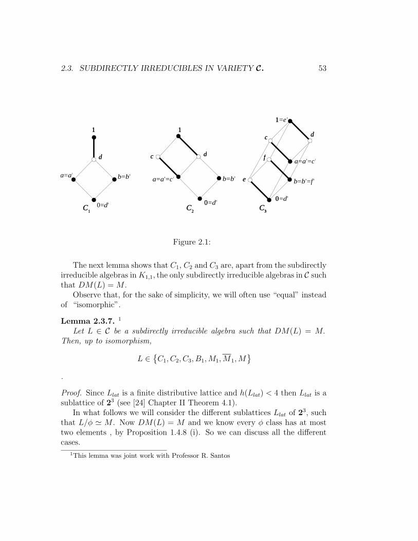
2.3. SUBDIRECTLY IRREDUCIBLES IN VARIETY C. 53
a=a’ b=b’
dd
0=d’CC11
11
CC33
00=d’
a=a’=c’
11=e’
cc
ee b=b’=f’
dd
ff
CC22
a=a’=c’ b=b’
dd
11
00=d’
cc
Figure 2.1:
The next lemma shows that C1, C2 and C3 are, apart from the subdirectlyirreducible algebras inK1,1, the only subdirectly irreducible algebras in C suchthat DM(L) = M .
Observe that, for the sake of simplicity, we will often use “equal” insteadof “isomorphic”.
Lemma 2.3.7. 1
Let L ∈ C be a subdirectly irreducible algebra such that DM(L) = M.Then, up to isomorphism,
L ∈{C1, C2, C3, B1,M1,M1,M
}.
Proof. Since Llat is a finite distributive lattice and h(Llat) < 4 then Llat is asublattice of 23 (see [24] Chapter II Theorem 4.1).
In what follows we will consider the different sublattices Llat of 23, suchthat L/φ ' M . Now DM(L) = M and we know every φ class has at mosttwo elements , by Proposition 1.4.8 (i). So we can discuss all the differentcases.
1This lemma was joint work with Professor R. Santos

54 CHAPTER 2. THE VARIETY C
As we did in Figure 2.1, we will denote by a and b the fixed points of L.
Case 1:Llat is 23.Every φ class has two elements, therefore we have the following possibil-
ities:(i) The fixed points are an atom and a co-atom.Then L is equal to B1.(ii) The fixed points are two atoms.Then we obtain C3.(iii) The fixed points are two co-atoms.In this case, L /∈ SDMA. In fact, supposing 0/φ = {0, e}, where
e = a ∧ b, we have a′′ ∧ b′′ = e 6= (a ∧ b)′′ = 0.
Case 2:Llat is the sublattice 2× 3 of 23.It is clear, since φ is a congruence relation in Llat, that exactly one of the
classes 0/φ and 1/φ has two elements and that exactly one of the classes a/φand b/φ has two elements.
We only need to consider the following subcases.(i) The fixed points are an atom and a co-atom.Assuming, without loss of generality, that a is a co-atom and b is an atom:If |1/φ| = 2 then |0/φ| = 1, |a/φ| = 2 and |b/φ| = 1. So we obtain M1. If
|1/φ| = 1 then |0/φ| = 2, |a/φ| = 1 and |b/φ| = 2. So we obtain M1.(ii) The fixed points are two atoms.In this case |0/φ| = 1 and |1/φ| = 2. Suppose without loss of generality
that |a/φ| = 2 then |b/φ| = 1 and we obtain C2.(iii) The fixed points are two co-atoms.In this case |1/φ| = 1, |0/φ| = 2. Using the same argument of Case 1
(iii), we conclude L 6∈ SDMA.
Case 3:Llat is the sublattice 22 ⊕ 1 or the sublattice 1⊕ 22 of 23.It is obvious that one and only one of the classes 0/φ and 1/φ has two
elements.If Llat = 22 ⊕ 1 then |1/φ| = 2, and we obtain C1
If Llat = 1⊕ 22 then |0/φ| = 2, and as in Case 1 (iii), L /∈ SDMA.
Case 4:Llat is the sublattice 22 of 23.

2.3. SUBDIRECTLY IRREDUCIBLES IN VARIETY C. 55
Clearly in this case we have L = M .
Theorem 2.3.8. Let L ∈ C . Then the following are equivalent:
(i) L is subdirectly irreducible.
(ii) L is a subdirectly irreducible demi p-lattice or L is a subdirectly irre-ducible algebra in the variety K1,1 of Ockham algebras or L is up toisomorphism in {C1, C2, C3}.
Proof. We first show (i) implies (ii). By Lemma 2.3.4 we know that if L ∈ Cis a subdirectly irreducible algebra then L is a subdirectly irreducible algebraof DMPL or DM(L) is a subdirectly irreducible algebra of DMA. In thiscase it results from Lemmas 2.3.6 and 2.3.7 that L is a subdirectly irreduciblealgebra in the variety K1,1 of Ockham algebras or L is up to isomorphism in{C1, C2, C3}.
It is trivial that (ii) implies (i).
In Figure 2.2 we present the diagrams of the finite subdirectly irreduciblealgebras of C: B0,2, K1, K1, K2 and S since they will be necessary in thenext section.
00
a=a’
ee
1=e’
_KK
22
aa
KK11
b=b’=a’
11
00
11
a=a’=b’
bb
00 _KK
11
__SS
00
1=e’
ee
a=b’ b=a’
dd
0=d’BB
0,2
11
Figure 2.2:
Sankappanavar proved in [40] Corollary 3.2 that every subalgebra of a sub-directly irreducible demi-p-lattice is also subdirectly irreducible. The same

56 CHAPTER 2. THE VARIETY C
is true in variety C, since this is true for the subalgebras of the subdirectlyirreducible algebras of K1,1 and for the subalgebras of C1, C2 and C3.
Corollary 2.3.9. If L ∈ C is a subdirectly irreducible algebra, then so isevery subalgebra of L.
The variety SDMA is known to be locally finite. A proof can be foundin Theorem 5.1 of [25]. It is also well known that this variety is congruence-distributive. These results together with a fundamental theorem reachedby Davey in [16] will help to describe a poset such that the lattice of itsdown-sets is isomorphic to the lattice of the subvarieties of variety C.
Let Λ (K) denote the lattice of subvarieties of a variety K and let SIF (K)be a set consisting of precisely one algebra from each of the isomorphismclasses of the nontrivial finite subdirectly irreducible algebras in the varietyK.
Theorem 2.3.10. (Davey [16], Theorem 3.3)Let K be a locally finite congruence-distributive variety and order the set
SIF (K) byL1 ≤ L2 if and only if L1 ∈ HS (L2) .
Then Λ (K) is a completely distributive lattice and is isomorphic to D (SIF (K)).
Sankappanavar described the poset SIF (DMPL) in [40] (see Definition6.7 (iii) and (iv), Lemma 6.8 and Corollary 6.10). In [9] page 91, the posetSIF (K1,1) is described so, using these results and Theorem 2.3.8, it is easyto obtain the Hasse diagram of the poset SIF (C).
With this aim we note that both in K1,1 and DMPL every non-trivialhomomorphic image of a finite subdirectly irreducible algebra L is isomorphicto a subalgebra of L (see [37] Corollary 2.9 and [40] Lemma 3.5.) so, for thesealgebras, L1 ∈ HS(L2) is equivalent to L1 ∈ IS(L2). This is not true forC1, C2 and C3. In fact, if L is in {C1, C2, C3} then L/φ ' M and M is notisomorphic to a subalgebra of L. Since for such an L, φ is the minimumelement of Con(L)\{∆}, it follows that, for any θ ∈ Con(L)\{∆, ∇}, L/θis a subdirectly irreducible algebra of DMA.
Thus, for L ∈ {C1, C2, C3}, we have L1 ≤ L if and only if L1 ∈ S(L) orL1 is a subdirectly irreducible De Morgan algebra.
We present the diagram of SIF (C) in Figure 2.3 where, as pointed in[40], B ⊂ S ⊂ B0,2 ⊂ · · · ⊂ B0,n ⊂ · · · is the chain of subdirectly irreduciblepseudocomplemented lattices.
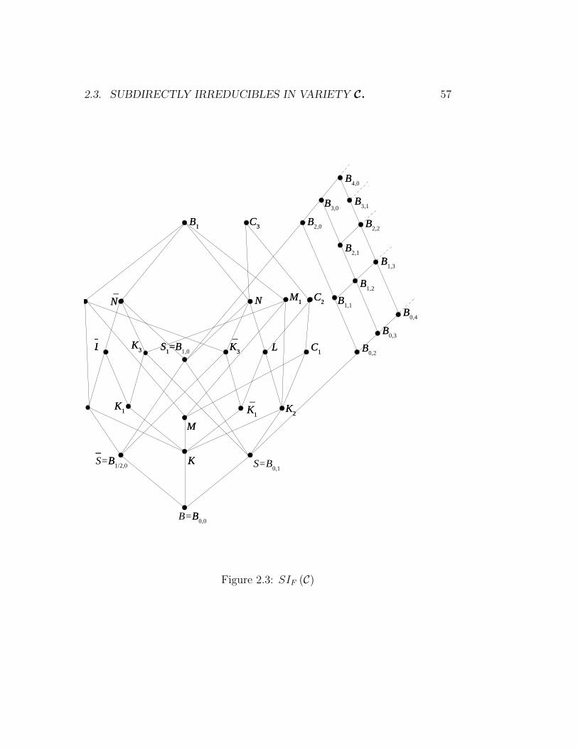
2.3. SUBDIRECTLY IRREDUCIBLES IN VARIETY C. 57
S=B0,1
KK22
LL
__S=BB
1/2,0KK
MM
_KK
33
_KK
11
_KK
22KK
11
SS11==BB
1,0 KK
33
__LL BB
0,2
__MM
11
_NN NN MM
11 BB1,1
BB2,0
BB11
CC22
CC33
CC11
BB0,4
BB3,0
BB2,1
BB1,2
BB0,3
BB4,0
BB3,1
BB2,2
BB1,3
B=BB0,0
Figure 2.3: SIF (C)

58 CHAPTER 2. THE VARIETY C
We can extend a result obtained by R. Beazer ([7] Corollary 7) for thevariety K1,1.
Corollary 2.3.11. Let L ∈ C \ DMA be a finite subdirectly irreduciblealgebra. Then Con(L)={∆, φ, ∇} if and only if L ∈ (K1,1 \ DMA) ∪{C1, C2, C3}.
Proof. Let L ∈ C \DMA be a finite subdirectly irreducible algebra.Suppose Con(L) = {∆, φ, ∇}. Clearly L /∈ DMA. Assume that L /∈
(K1,1 \ DMA) ∪ {C1, C2, C3}. Then by the diagram of Figure 2.3 we havethat L contains B0,2 as a subalgebra. Since Con(B0,2) = 1⊕ 22 and DMPLsatisfies CEP it is obvious |Con(L)| > 3, a contradiction.
If L ∈ (K1,1 \DMA)∪{C1, C2, C3} then by Theorem 2.3.8 L/φ is simpleand ∆ 6= φ so Con(L) = {∆, φ, ∇}.
2.4 Equational Bases for some Subvarieties.
In this section we describe equational bases for the subvarieties of C generatedby C1, by C2 and by C3.
Note that K1,1 is characterized, as a subvariety of C, by the identity(a ∧ b)′ = a′ ∨ b′. So, when we consider each subvariety V of K1,1, generatedby a single subdirectly irreducible algebra, as a subvariety of C we only needto add to this identity the equational bases characterizing V as a subvarietyof K1,1. These equational bases are presented in [37] and [9].
If L ∈ C then V(L) denotes the variety generated by L. Please read“defined by” as “defined, modulo C, by”.
While reading the proofs of the following theorems it might be useful torefer to Figures 2.2 and 2.3
Theorem 2.4.1. V (C3) is defined by
(λ) a′ ∧ a′′ ≤ a ∧ a′.
(µ) a ∧ a′ ∧ b′′ ∧ b′ = b ∧ b′ ∧ a′′ ∧ a′.
(ξ) a′ ∨ a′′ = (a′ ∧ a)′.
Proof. Observe V (C3) |= (λ), (µ) , and (ξ), B0,2 6|= (ξ) because a′ ∨ a′′ = dand (a′ ∧ a)′ = 1, K1 6|= (λ) because a∧a′ = a and a′′∧a′ = b and K2 6|= (µ)because e ∧ e′ ∧ a′′ ∧ a′ = e and a ∧ a′ ∧ e′′ ∧ e′ = 0.

2.4. EQUATIONAL BASES FOR SOME SUBVARIETIES. 59
Also observe that if L is a finite subdirectly irreducible algebra in C andL /∈ HS (C3) then L contains, up to isomorphism, B0,2 or K1 or K2 assubalgebras. Thus, if V is the subvariety of C defined by (λ), (µ) and (ξ),then SIF (V) = HS (C3) so V = V (C3).
Theorem 2.4.2. V (C2) is defined by(ξ) a′ ∨ a′′ = (a′ ∧ a)
′.
(ρ) a ∧ a′ = a′′ ∧ a′.
Proof. Observe V (C2) |= (ξ) and (ρ), B0,2 6|= (ξ) because a′ ∨ a′′ 6= (a′ ∧ a)′ ,K1 6|= (ρ) because a ∧ a′ 6= a′′ ∧ a′ and S 6|= (ρ) because e ∧ e′ 6= e′′ ∧ e′.
If L is a finite subdirectly irreducible algebra in C and L /∈ HS (C2) thenL contains, up to isomorphism, B0,2 or K1 or S as subalgebras. Thus, if Vis the subvariety of C defined by (ξ),and (ρ), then SIF (V) = HS (C2) soV = V (C2).
Theorem 2.4.3. V (C1) is defined by(ξ) a′ ∨ a′′ = (a′ ∧ a)
′.
(ρ) a ∧ a′ = a′′ ∧ a′.(σ) a ≤ a′′.
Proof. Observe V (C1) |= (ξ), (ρ) and (σ), B0,2 6|= (ξ), K1 6|= (ρ) and S 6|= (ρ)as we saw in the previous theorem, and K1 6|= (σ) because b′′ < b.
If L is a finite subdirectly irreducible algebra in C and L /∈ HS (C1) thenL contains, up to isomorphism, B0,2 or K1 or K1 or S as subalgebras. Thus,if V is the subvariety of C defined by (ξ), (ρ) and (σ), then SIF (V) = HS (C1)so V = V (C1).

60 CHAPTER 2. THE VARIETY C

Chapter 3
Duality
We develop here a duality based on the theory of canonical extensions. Theidea is that dualities are extracted by composing canonical extension andcorrespondence for complex algebras. This is a general program which thispaper will illustrate.
3.1 Canonical extension and canonicity
3.1.1 Canonical extensions of Distributive Lattices
We will describe here some results on canonical extensions of bounded dis-tributive lattices (DL) obtained by M. Gehrke and B. Jonsson in [18], [19]and [20] and by M. Gehrke, H. Nagahashi and Y. Venema in [21].
In the interest of self containment we list here some important facts.
For a lattice L, we will denote by J∞(L) the set of all completely joinirreducible elements of L and by M∞(L) the set of all completely meet irre-ducible elements of L. By J∞ω (L) and M∞
ω (L) we denote the sets consisting,respectively, of all finite joins of elements of J∞(L) and all finite meets ofelements of M∞(L). Observe that 0 ∈ J∞ω (L) but 0 /∈ J∞(L) and that1 ∈ M∞
ω (L) but 1 /∈ M∞(L). For convenience we set J∞0 (L) = J∞(L) ∪ {0}and M∞
1 (L) = M∞(L) ∪ {1}.
Definition 3.1.1. ([21] Definition 2.12, [20] Definition 2.4)Suppose L is a bounded sublattice of a complete lattice L′. We say that
61

62 CHAPTER 3. DUALITY
1. L is dense in L′ if every element of L′ can be expressed both as a joinof meets and as a meet of joins of elements from L.
2. L is separating in L′ if for all p, q ∈ J∞(L′) with p 6≤ q there existsa ∈ L such that q ≤ a and p 6≤ a.
3. L is compact in L′ if, for all S, T ⊆ L with∧S ≤
∨T in L′, there
exist finite sets F ⊆ S and G ⊆ T such that∧F ≤
∨G.
For a bounded distributive lattice L, the lattice of clopen down-sets of thedual Priestley space (X,≤, τ) is dense and compact in the complete lattice ofdown-sets of (X,≤) . On the other hand, one can show that between any twocomplete extensions of L that satisfy these two conditions there is a uniqueisomorphism so the following definition makes sense:
Definition 3.1.2. ([21] Definition 2.13)The canonical extension of a DL L is a complete lattice Lσ containing L
as a dense and compact sublattice.
And we have also the following,
Theorem 3.1.3 ([20]Theorem 2.5. (i)). If L is a DL, then Lσ containsL as a separating sublattice.
Let L ∈ DL. We will often use the lattice obtained from L by reversingthe order which we call the (order) dual lattice of L.
Definition 3.1.4. ([21] Definition 2.10)Given a bounded distributive lattice L = (L,∨,∧, 0, 1), let L∂ denote
the dual lattice, that is, the structure L∂ = (L,∧,∨, 1, 0). For technicalconvenience, let L1 = L.
An element ε ∈ {1, ∂}n is called an order type; the i-th component ofsuch an ε will be denoted by εi.
Given an order type ε ∈ {1, ∂}n, let Lε denote Lε1 × ...× Lεn .
Obviously L and L∂ have the same universe. Since the characterizationof canonical extensions is self-dual it is possible to identify (Lσ)∂ with (L∂)σ
([19] Corollary 3).We always have J∞(L∂) = M∞(L) and M∞(L∂) = J∞(L).
The canonical extension of a distributive lattice is a perfect distributivelattice.

3.1. CANONICAL EXTENSION AND CANONICITY 63
Definition 3.1.5. ([21] Definition 2.14)A distributive lattice L is called perfect or a DL+ if it satisfies one of the
following, equivalent, conditions:1. L is doubly algebraic (that is, both L and L∂ are algebraic).2. L is complete, completely distributive and join generated by the set
J∞(L)3. L is isomorphic to a set-theoretic lattice based on the collection of
down-sets of some partially ordered set.
Note that, since condition 1 is self-dual, the duals of conditions 2 and 3also hold for perfect distributive lattices.
As is mentioned in [21], the density of L in Lσ implies that J∞(Lσ) iscontained in K(Lσ), the meet closure of L in Lσ, and M∞(Lσ) is containedin O(Lσ), the join closure of L in Lσ.
Since the canonical extension of a bounded distributive lattice can beobtained by taking the poset of all order ideals or down-sets of its topo-logical dual space, we refer to elements of L as clopen elements, to elementsof K(Lσ) as closed elements and to elements of O(Lσ) as open elements of Lσ.
If L is a perfect distributive lattice, there is a natural isomorphism be-tween the posets J∞(L) and M∞(L).
Definition 3.1.6. ([20] Definition 2.2)Given a lattice L ∈ DL+ we define
(i) κ(p) =∨
(L \ (↑ p)) for all p ∈ J∞(L).
(ii) κ−1(u) =∧
(L \ (↓ u)) for all u ∈M∞(L).
Theorem 3.1.7 ([20] Theorem 2.3 ). For any L ∈ DL+,
κ : (J∞(L),≤) ' (M∞(L),≤) : κ−1
i.e., κ is an isomorphism from the poset J∞(L) onto the poset M∞(L) andκ−1 is the inverse of κ.
Remark 3.1.8. Observe that this isomorphism is such that, for any a ∈ Land any p ∈ J∞(L),
p 6≤ a ⇔ κ(p) ≥ a.
64 CHAPTER 3. DUALITY
A map f : L → K between L,K ∈ DL can be extended in various waysto a map between Lσ and Kσ.
In order to define the extensions of a map f , six topologies will be intro-duced here.
Definition 3.1.9. ([20] Definition 2.6.)Suppose L ∈ DL. We denote by σ, σ↑ and σ↓ the topologies on Lσ having
as bases, respectively, the open sets of the forms ↑ p∩ ↓ u, ↑ p and ↓ u, withp ∈ K(Lσ) and u ∈ O(Lσ).
The other three topologies will be defined in the same manner, except thatnow the elements p and u are, respectively, compact and dually compact inthe lattice theoretic sense and thus these topologies can be defined in anarbitrary doubly algebraic distributive lattice K.
Definition 3.1.10. ([20] Definition 2.7)Suppose K is a doubly algebraic lattice. We denote by ι, ι↑ and ι↓ the
topologies on K having as bases, respectively, the open sets of the forms↑ p∩ ↓ u, ↑ p and ↓ u, with p compact and u dually compact.
Observe that the elements of J∞ω (K) are the compact elements in thesense of lattice theory and the members of M∞
ω (K) are the dually compactelements and that it follows that sets of the form ↑ p∩ ↓ u, ↑ p and ↓ u, withp ∈ J∞(K) and u ∈ M∞(K) form subbases for the topologies ι, ι↑ and ι↓,respectively.
Obviously, the topology σ is the join of σ↑ and σ↓ and ι is the join of ι↑
and ι↓.For any L ∈ DL, the topologies ι, ι↑ and ι↓ on Lσ are weaker than σ, σ↑
and σ↓, respectively, because J∞ω (Lσ) ⊆ K(Lσ) and M∞ω (Lσ) ⊆ O(Lσ).
In general, if we have sets X and Y with topologies τ and µ and if themap g : X → Y is continuous relatively to τ on X and µ on Y we say thatg is (τ, µ)-continuous.
Remark 3.1.11. Since continuity only needs to hold on a subbase we have:The map g : Lσ → Kσ is (σ, ι↑)-continuous means that, for all u ∈ Lσ and
for all q ∈ J∞(Kσ), if q ≤ g(u) then there exist K(Lσ) 3 x ≤ u ≤ y ∈ O(Lσ)so that q ≤ g(v) for all v ∈ Lσ such that x ≤ v ≤ y.
And:

3.1. CANONICAL EXTENSION AND CANONICITY 65
The map g is (σ, ι↓)-continuous means that, for all u ∈ Lσ and for alln ∈ M∞(Kσ), if n ≥ g(u) then there exist K(Lσ) 3 x ≤ u ≤ y ∈ O(Lσ) sothat n ≥ g(v) for all v ∈ Lσ such that x ≤ v ≤ y.
Now we will describe the canonical extensions of arbitrary maps betweendistributive lattices and we will consider the continuity of these maps.
Definition 3.1.12. ([21] Definition 2.15)Suppose L,K ∈ DL. Given a map f : L→ K we define two maps
fσ, fπ : Lσ −→ Kσ
by
fσ(u) =∨{∧
{f(a) : a ∈ L and x ≤ a ≤ y} : K(Lσ) 3 x ≤ u ≤ y ∈ O(Lσ)}
and
fπ(u) =∧{∨
{f(a) : a ∈ L and x ≤ a ≤ y} : K(Lσ) 3 x ≤ u ≤ y ∈ O(Lσ)}
for each u ∈ Lσ .
As proved in [20] Theorem 2.12 we have the following topological charac-terization of fσ and fπ:
Theorem 3.1.13. For any map f : L → K with L,K ∈ DL, the mapsfσ and fπ are extensions of f . In fact, fσ is the largest (σ, ι↑)-continuousextension of f to Lσ and fπ is the smallest (σ, ι↓)-continuous extension of fto Lσ.
From [20] Theorem 2.11 (iii) it follows:
Corollary 3.1.14. For any map f : L → K with L,K ∈ DL, the maps fσ
and fπ are such that fσ ≤ fπ.
Maps f for which fσ = fπ are particularly nice. These maps are calledsmooth and we have:
Corollary 3.1.15 ([20]Corollary 2.17). If f : L→ K is smooth, then theextension fσ = fπ of f is (σ, ι)-continuous. Conversely, if f has a (σ, ι)-continuous extension g : Lσ → Kσ, then f is smooth and fσ = fπ = g.

66 CHAPTER 3. DUALITY
Remark 3.1.16. If the map f : L → K is isotone then, from [20] Corollary2.19, it follows that the descriptions of fσ and fπ can be simplified . Thenfor all u ∈ Lσ
fσ(u) =∨{∧
{f(a) : a ∈ L and x ≤ a} : K(Lσ) 3 x ≤ u)}
and
fπ(u) =∧{∨
{f(a) : a ∈ L and a ≤ y} : u ≤ y ∈ O(Lσ)}.
Also, for all x ∈ K(Lσ) and y ∈ O(Lσ),
fσ(x) = fπ(x) =∧{f(a) : a ∈ L and x ≤ a},
fπ(y) = fσ(y) =∨{f(a) : a ∈ L and a ≤ y}.
So, fσ and fπ agree on closed and open elements .
Remark 3.1.17. For isotone maps, the (σ, ι↑)-continuity of fσ yields the(σ↑, ι↑)-continuity of fσ.
This continuity may be stated as follows and was in fact already identifiedin this non-topological guise in [18]:
Lemma 3.1.18 ([18]Corollary 3.9). Suppose f : L→ K, with L,K ∈ DL,is isotone and p ∈ J∞(Kσ). Below every element u ∈ Lσ that satisfies theinclusion p ≤ fσ(u) there is a minimal solution of this inclusion, and all theminimal solutions are closed elements.
When composing isotone maps we have:
Theorem 3.1.19 ([19] Theorem 15). Let g : L1 → L2 and f : L2 → L3
be isotone maps on DLs. If g is meet preserving then (f ◦ g)σ = fσ ◦ gσ.Dually, if g is join preserving, then (f ◦ g)π = fπ ◦ gπ.
Some special maps play an important part in our study so we will seehow they behave in what concerns canonical extensions. To do so we haveto give the following:
Definition 3.1.20. Let L,K ∈ DL+ and let {ai : i ∈ I} be any subset ofL. We say that a map f : L→ K is:

3.1. CANONICAL EXTENSION AND CANONICITY 67
(i) completely join preserving, if f(0) = 0 and f(∨
i∈I ai
)=∨
i∈I f(ai).
(ii) completely meet preserving, if f(1) = 1 and f(∧
i∈I ai
)=∧
i∈I f(ai).
(iii) completely join reversing, if f(0) = 1 and f(∨
i∈I ai
)=∧
i∈I f(ai).
(iv) completely meet reversing, if f(1) = 0 and f(∧
i∈I ai
)=∨
i∈I f(ai).
Properties of join preserving maps were studied first [18]. Then theywere generalized to the other cases by using properties of the order dual of adistributive lattice.
Remark 3.1.21. ([21] Remark 2.11)Given L,K ∈ DL and two order types (Definition 3.1.4) ε and ε′, if we
consider two maps f : Lε → K and g : Lε′ → K that are set-theoreticallyidentical (that is f(a) = g(a) for all a ∈ Ln), such maps will be called ordervariants.
Observe that, from the definition of fσ and gσ, if f and g are order vari-ants then so are fσ and gσ and these maps are also set-theoretically identical.Clearly, the same is also true for fπ and gπ.
Dualizing the order in the codomain however does make a difference. Infact, given a map f : L→ K, denoting by f∂ the same set-theoretic map asf but with the order dualized on both domain and codomain, f∂ : L∂ → K∂,it is easy to see, from the definitions of fσ and fπ, that (f∂)σ = (fπ)∂ and(f∂)σ = (fπ)∂.
Therefore, if a map f is smooth both its order variants and f∂ are smooth,and either extension of any order variant of f and f∂ all give the same settheoretic function.
Using these properties it is possible to prove:
Lemma 3.1.22 ([19]Theorem 10, [20]Corollary 2.28). If the map f :L→ K, with L,K ∈ DL, is a join preserving map then fπ is completely joinpreserving, if f is meet preserving then fσ is completely meet preserving.
In either case f is smooth.
and
Lemma 3.1.23 ([21] page 12, [20] Theorem 2.23). Let L,K ∈ DL.If the map f : L→ K is a join reversing (or meet reversing) map then fσ
is completely join reversing (or meet reversing). In either case f is smooth.

68 CHAPTER 3. DUALITY
3.1.2 Canonical extensions of Distributive Algebras
We will now consider algebras having as a reduct a bounded distributivelattice and unary operations that are meet or join preserving or meet orjoin reversing. These were called Distributive Modal Algebras (DMA) in[21] where they were considered as algebraic counterparts to DistributiveModal Logics. However, as our main object of study here will be semi-DeMorgan Algebras which contain the De Morgan Algebras (DM) or (DMA),these latter algebras could easily be confused with the Distributive ModalAlgebras. In [22], operations that turn joins or meets in any one coordinate tojoins (meets) are called (dual) quasi-operators and thus we will use the nameUnary quasi-operators algebras, UQA, instead of DMA for these algebraswhich consist of a distributive lattice with additional operations that areunary quasi-operators or unary dual quasi-operators.
Definition 3.1.24. Let UQA be the class of algebras
(L,∧,∨, 0, 1,3,2,B,C)
such that (L,∧,∨, 0, 1) is a bounded distributive lattice, and 3,2,B,C areunary operations such that for any a, b ∈ L:
(i) 30 = 0 and 3(a ∨ b) = 3a ∨3b.
(ii) 21 = 1 and 2(a ∧ b) = 2a ∧2b.
(iii) B 0 = 1 and B (a ∨ b) =B a∧ B b.
(iv) C 1 = 0 and C (a ∧ b) =C a∨ C b.
Let Lσ be the canonical extension of L. The operations 3σ and 3π aresuch that, for each u ∈ Lσ,
3σ(u) =∨{∧{3a : x ≤ a ∈ L} : u ≥ x ∈ K(Lσ)}
3π(u) =∧{∨{3a : y ≥ a ∈ L} : u ≤ y ∈ O(Lσ)}.
Since all maps that preserve joins are smooth (Lemma 3.1.22), we have3σ = 3π.
Similarly, the other unary operations can be extended to Lσ and all theseextensions are smooth so it makes sense the following definition:

3.1. CANONICAL EXTENSION AND CANONICITY 69
Definition 3.1.25 ([21] Definition 2.19). Let (L, ,∧,∨, 0, 1,3,2,B,C) ∈UQA. The canonical or perfect extension of L is the algebra
(Lσ,∧,∨, 0, 1,3σ,2σ,Bσ,Cσ) = (Lσ,∧,∨, 0, 1,3π,2π,Bπ,Cπ).
From Lemma 3.1.22 and subsequent remarks we can conclude that thesecanonical extensions satisfy the conditions of the following definition:
Definition 3.1.26. Let UQA+ be the class of algebras
(L,∧,∨, 0, 1,3,2,B,C)
such that (L,∧,∨, 0, 1) ∈ DL+, and 3,2,B,C are unary operations suchthat for any subset {ai : i ∈ I} ⊆ L:
(i) 30 = 0 and 3
(∨i∈I
ai
)=∨i∈I
3ai.
(ii) 21 = 1 and 2
(∧i∈I
ai
)=∧
2ai.
(iii) B 0 = 1 and B
(∨i∈I
ai
)=∧i∈I
B ai.
(iv) C 1 = 0 and C
(∧i∈I
ai
)=∨i∈I
C ai.
So,
Lemma 3.1.27 ([21] Lemma 2.21). If L is a UQA then Lσ is a UQA+.
In what concerns UQA-homomorphisms observe that UQA-algebras arein the scope of the following definitions:
Definition 3.1.28. ([21] Definition 5.4 )A Distributive Lattice Expansion is any algebra (L, (fi)i∈I) consisting of
a DL, L = (L,∨,∧, 0, 1), and additional operations fi : Lni → L for eachi ∈ I. Such an algebra is said to be monotone provided each basic operationis monotone, that is, for each i ∈ I, there is an order type εi ∈ {1, ∂}ni
so that fi : Lεi → L is order preserving. The sequence (εi)i∈I is called themonotonicity type of L.

70 CHAPTER 3. DUALITY
For these algebras we have (from [20] Lemma 3.24 ) thatEvery homomorphism h : L → K where L,K are monotone is preserved
by canonical extensions. Even more, hσ : Lσ → Kσ is a complete homomor-phism.
So we can conclude that σ is a functor from the category of all UQAsand their homomorphisms into the category of all UQA+s and their completehomomorphisms.
Remark 3.1.29. It is clear that these results apply to algebras that are reductsof UQAs.
Properties that are preserved by canonical extensions are of great interest.Such properties will be called canonical.
Definition 3.1.30. ([21] Definition 2.22)A class of UQAs is canonical if it is closed under taking canonical exten-
sions.An equation, formula or set of formulas is called canonical if the class of
UQAs defined by the equation, formula or set of formulas is canonical.
3.1.3 Sahlqvist inequalities and canonicity
Not all the properties in a UQA are canonical, but a broad class of canonicalinequalities, called Sahlqvist inequalities, was identified for unary Booleanalgebras with operators in [35] and for UQAs in [21]. The definitions in [21]were given for so-called sequents, but we will give them here for the corre-sponding inequalities.
With each term for UQAs associate two generation trees, the positiveand the negative generation tree, depending on whether the sign of the rootis (+) and (−), respectively. Each of these will be an expansion of the term’sgeneration tree in which every node is signed with either + or −. Thesesignings are required to satisfy the following constraints:
• If a node is ∨,∧,3 or 2, assign the same sign to its successor nodes.
• If a node is C or B, assign the opposite sign to its successor node.
By these conditions, the sign of each node is determined by the sign of theroot of the tree. Thus with each term we may associate two signed generation
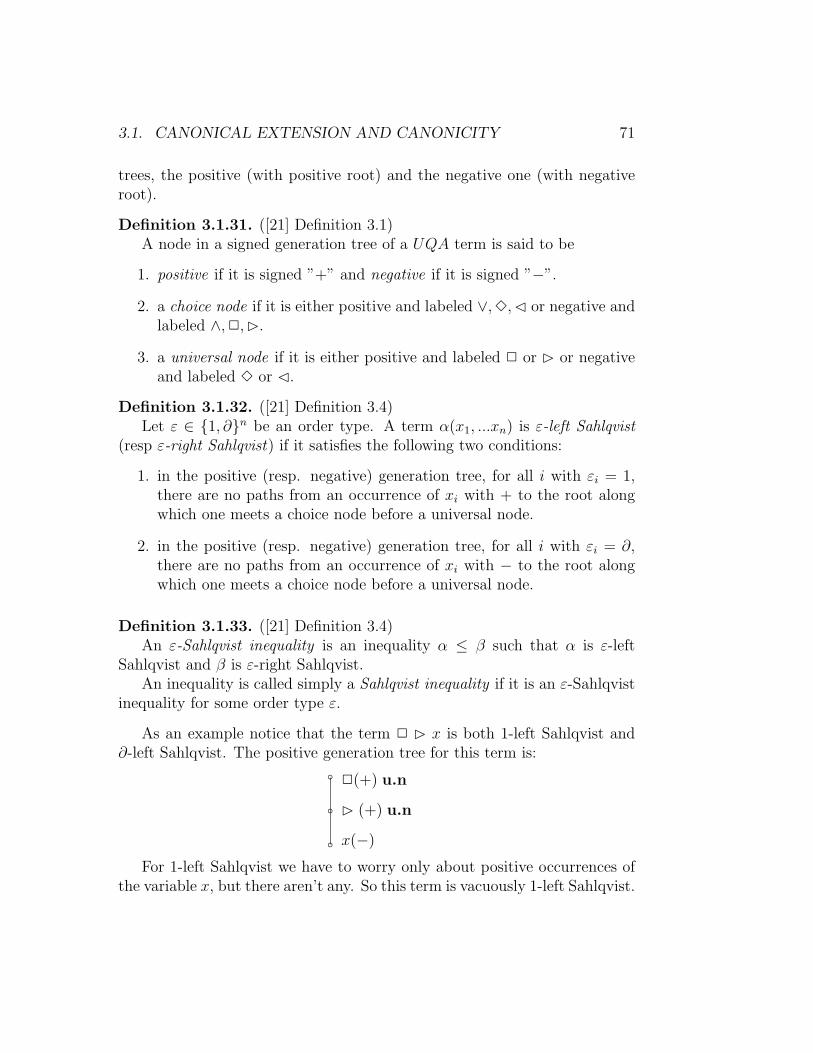
3.1. CANONICAL EXTENSION AND CANONICITY 71
trees, the positive (with positive root) and the negative one (with negativeroot).
Definition 3.1.31. ([21] Definition 3.1)A node in a signed generation tree of a UQA term is said to be
1. positive if it is signed ”+” and negative if it is signed ”−”.
2. a choice node if it is either positive and labeled ∨,3,C or negative andlabeled ∧,2,B.
3. a universal node if it is either positive and labeled 2 or B or negativeand labeled 3 or C.
Definition 3.1.32. ([21] Definition 3.4)Let ε ∈ {1, ∂}n be an order type. A term α(x1, ...xn) is ε-left Sahlqvist
(resp ε-right Sahlqvist) if it satisfies the following two conditions:
1. in the positive (resp. negative) generation tree, for all i with εi = 1,there are no paths from an occurrence of xi with + to the root alongwhich one meets a choice node before a universal node.
2. in the positive (resp. negative) generation tree, for all i with εi = ∂,there are no paths from an occurrence of xi with − to the root alongwhich one meets a choice node before a universal node.
Definition 3.1.33. ([21] Definition 3.4)An ε-Sahlqvist inequality is an inequality α ≤ β such that α is ε-left
Sahlqvist and β is ε-right Sahlqvist.An inequality is called simply a Sahlqvist inequality if it is an ε-Sahlqvist
inequality for some order type ε.
As an example notice that the term 2 B x is both 1-left Sahlqvist and∂-left Sahlqvist. The positive generation tree for this term is:
x(−)bb B (+) u.n
b2(+) u.n
For 1-left Sahlqvist we have to worry only about positive occurrences ofthe variable x, but there aren’t any. So this term is vacuously 1-left Sahlqvist.

72 CHAPTER 3. DUALITY
For ∂-left Sahlqvist, we have to worry about negative occurrences of x.There is one, but since all nodes in the tree are universal, there is no problemanyway. Thus this term is also ∂-left Sahlqvist.
So the inequality 2 B x ≤ x is Sahlqvist.For Sahlqvist inequalities we have the following:
Theorem 3.1.34 ([21] Theorem 5.1). Every Sahlqvist inequality is canon-ical in UQA.

3.2. DISCRETE DUALITY 73
3.2 Discrete Duality
3.2.1 Basic technical ingredients
Correspondence between Perfect Lattices and Posets
A correspondence between the class of Perfect Distributive Lattices (Defini-tion 3.1.5) and Posets was studied by G. Raney [34], V. Balachandran [3] andP. Dwinger [4]. More recently S.T.Thomason [42]and M.Gehrke, H.Nagashiand Y. Venema ( [21]) have extended this correspondence in order to obtaina duality that generalizes Birkhoff’s duality for finite distributive lattices.
Let L be a DL+ (Definition 3.1.5). The lattice L gives rise to a poset(J∞(L),≤) where J∞(L) is the set of completely join irreducible elements ofL and ≤ is the restriction to J∞(L) of the order in the lattice L. In turn, foran arbitrary poset X, let (D(X),∩,∪, ∅, X) be the lattice of downsets of X.Then this lattice is in DL+. So, denoting by P posets (X,≤), we can definemaps
()+ : DL+ → P such that (L)+ = J∞(L) for each L ∈ DL+
and
()+ : P → DL+ such that (X)+ = D(X) for each X ∈ P .
In Theorem 2 [34] G.Raney proved that for a complete distributive latticeL to be isomorphic to the lattice of downsets of J∞(L) it is necessary andsufficient that every element of L is the join of a set of completely joinirreducible elements. From the proof of this theorem it follows:
Theorem 3.2.1. The maps ()+ : DL+ → P and ()+ : P → DL+ are suchthat, for each L ∈ DL+, there is an isomorphism ηL : L → ((L)+)+ definedby
ηL(a) = {x ∈ J∞(L) : x ≤ a} (= J∞(L)∩ ↓ a)
for any a ∈ L.
On the other hand, for an arbitrary poset X, the completely join irre-ducible elements of the lattice (D(X),∩,∪, ∅, X) are exactly the principaldownsets, ↓ x with x ∈ X, so we have:
74 CHAPTER 3. DUALITY
Theorem 3.2.2. The maps ()+ : DL+ → P and ()+ : P → DL+ are suchthat for each X ∈ P there is an order isomorphism εX : X → ((X)+)+ where
εX(x) =↓ x
for any x ∈ X.
From the previous theorems it follows that the maps ()+ and ()+ deter-mine, at the objects level, a duality between the categories DL+ and P .
We want to extend these maps in order to obtain a duality so, we haveto define the morphisms of these categories.
Correspondence between maps and order compatible relations
Naturally morphisms of DL+ are complete homomorphisms. Morphisms ofP are order preserving maps. However, since we also have in mind extendingthe DL+s by additional operations and this will require that we produceduals for these, we will start by considering separately maps that preservearbitrary joins and maps that preserve arbitrary meets.
We will obtain the duality between DL+- morphisms and P-morphismsand we will determine the correspondents of unary operations that are join(meet) preserving as a corollary to this more general correspondence.
Let L,K ∈ DL+ and let f : L→ K be a completely join preserving map(Definition 3.1.20).
Let (X,≤X) and (Y,≤Y ) be posets such thatX = J∞(L) and Y = J∞(K)with the order induced from L and K, respectively.
The map f is uniquely determined by its value on the completely joinirreducible elements of L, J∞(L). In fact, since L is join generated by J∞(L),for any a ∈ L we have a =
∨p≤La p with p ∈ J∞(L) so
f(a) = f
( ∨p≤La
p
)=∨
p≤La
f(p). (3.2.1)
It would be convenient if we could define a binary relation S on the posetY ×X encoding f .

3.2. DISCRETE DUALITY 75
We cannot take S to be {(f(p), p) : p ∈ X} since, in general, f won’tmap into Y but, for each p ∈ X, we have
f(p) =∨q∈Y
q≤Kf(p)
q
since f(p) ∈ K and K is join generated by Y .Therefore we take S ⊆ Y ×X such that,
S = {(q, p) : q ≤K f(p)}.
The map f is order preserving, hence we have
≤Y ◦S◦ ≤X⊆ S.
On the other hand if we have posets (X,≤X) and (Y,≤Y ) and a relationS ⊆ Y ×X such that ≤Y ◦S◦ ≤X⊆ S, it is easy to prove that the map
fS : D(X)→ D(Y )
such that, for any U ∈ D(X),
fS(U) = S−1(U) = {q ∈ Y : ∃s ∈ U qSs}
is a completely join preserving map.Since there is no danger of misunderstanding, in what follows we will
denote the order relation by ≤ no matter the poset we are considering.Thus we have established the following:
Lemma 3.2.3. Let L,K ∈ DL+ and (X,≤) and (Y,≤) be the posets ofcompletely join irreducible elements of L and K, respectively. Then, to anycompletely join preserving map f : L→ K corresponds a binary relation
S = {(q, p) : q ≤ f(p)} ⊆ Y ×X
such that ≤ ◦S◦ ≤⊆ S.Conversely, if (X,≤) and (Y,≤) are posets and S ⊆ Y × X is a binary
relation such that ≤ ◦S◦ ≤⊆ S, then the map fS : D(X)→ D(Y ) defined by
fS(U) = S−1(U),
for every U ∈ D(X), is a completely join preserving map.

76 CHAPTER 3. DUALITY
In a way similar to the one we used for completely join preserving mapswe can determine the relation corresponding to a completely meet preservingmap.
To do this, given L ∈ DL+, we will often use the order dual lattice L∂.It follows from the definition of this lattice that M∞(L∂) = J∞(L) andJ∞(L∂) = M∞(L).
We will also use the order isomorphism κ : J∞(L)→M∞(L) (Definition3.1.6).
Since L ∈ DL+ is meet generated by the completely meet preservingelements, we have L∂ dually join generated by κ(J∞(L)). So, for any a ∈ L∂,
a =∧
p∈J∞(L)κ(p)≥a
κ(p) =∂∨
κ(p)∈J∞(L∂)κ(p)≤∂a
κ(p).
Let g : L→ K be a completely meet preserving map (Definition 3.1.20).If we consider the map
g∂ : L∂ → K∂.
This map is set theoretically identical to g and it is a completely join pre-serving map.
In fact for any a ∈ L,
g(a) = g∂
∂∨κ(p)∈J∞(L∂)
κ(p)≤∂a
κ(p)
=∂∨
κ(p)∈J∞(L∂)κ(p)≤∂a
g∂(κ(p)) =∧
p∈J∞(L)κ(p)≥a
g(κ(p)).
(3.2.2)Consequently g is uniquely determined by its value on κ(J∞(L)).Since, for any p ∈ J∞(L), g(κ(p)) is inK and this lattice is meet generated
by M∞(L) = κ(J∞(L)), we have:
g(κ(p)) =∧
q∈J∞(K)κ(q)≥g(κ(p))
κ(q).
Now we take T ⊆ J∞(K)× J∞(L) to be
T = {(q, p) : κ(q) ≥ g(κ(p)}

3.2. DISCRETE DUALITY 77
and T is such that:≤∂ ◦T◦ ≤∂⊆ T
which is equivalent to≥ ◦T◦ ≥⊆ T.
If we have posets (X,≤) and (Y,≤) and a relation T ⊆ Y ×X such that≥ ◦T◦ ≥⊆ T , then the map
gT : D(X)→ D(Y )
such that, for every U ∈ D(X),
gT (U) = X \ T−1(X \ U) = {q ∈ Y : ∀s ∈ X (qTs⇒ s ∈ U)}
is a completely meet preserving map.This way we obtain:
Lemma 3.2.4. Let L,K ∈ DL+ and (X,≤) and (Y,≤) be the posets ofcompletely join irreducible elements of L and K, respectively. Then, to anycompletely meet preserving map g : L→ K corresponds a binary relation
T = {(q, p) : κ(q) ≥ g(κ(p))} ⊆ Y ×X
such that ≥ ◦T◦ ≥⊆ T .If (X,≤) and (Y,≤) are posets and T ⊆ Y ×X is a binary relation such
that ≥ ◦T◦ ≥⊆ T , then the map gT : D(X)→ D(Y ) defined by
gT (U) = X \ T−1(X \ U),
for every U ∈ D(X), is a completely meet preserving map.
Now it is time to see what happens to complete homomorphisms h : L→K with L,K ∈ DL+.
We will follow the process used for endomorphisms in [21] 6.2.It is possible to consider h as a completely join preserving map f such
that f = g where g is completely meet preserving. Then f and g have tosatisfy
∀a ∈ L : f(a) ≤ g(a) and g(a) ≤ f(a).

78 CHAPTER 3. DUALITY
These inequalities are equivalent to conditions on the corresponding re-lations S and T .
To determine these conditions we are going to follow an algebraic methodthat will be often used in this chapter. This method consists in eliminatingthe universal quantifier on elements of L.
Condition ∀a ∈ L : f(a) ≤ g(a) is equivalent to:
∀a ∈ L∀q ∈ J∞(K) : (q ≤ f(a)⇒ q ≤ g(a)) (*)
because K is join generated by J∞(K).Now, from equation (3.2.1) and the fact that q is completely join irre-
ducible we conclude that q ≤ f(a) is equivalent to
∃p ∈ J∞(L) : (p ≤ a and q ≤ f(p)).
It follows, from the definition of S (Lemma 3.2.3), that this is equivalent to
∃p ∈ J∞(L) : (p ≤ a and qSp)
From equation (3.2.2), q ≤ g(a) is equivalent to
∀r ∈ J∞(L) : (κ(r) ≥ a⇒ q ≤ g(κ(r)))
and to∀r ∈ J∞(L) : (q 6≤ g(κ(r))⇒ κ(r) 6≥ a.)
From Remark 3.1.8 and the definition of T (Lemma 3.2.4) we obtain thefollowing equivalent expressions:
∀r ∈ J∞(L) : (g(κ(r)) ≤ κ(q)⇒ r ≤ a)
and∀r ∈ J∞(L) : (qTr ⇒ r ≤ a.)
Therefore, condition (*) is equivalent to
∀a ∈ L∀q ∈ J∞(K) :
((∃p ∈ J∞(L)(p ≤ a and qSp)) ⇒ (∀r ∈ J∞(L) : (qTr ⇒ r ≤ a)).
and to
∀a ∈ L∀q ∈ J∞(K)∀p, r ∈ J∞(L) : ((p ≤ a and qSp)⇒ (qTr ⇒ r ≤ a)).

3.2. DISCRETE DUALITY 79
Now observe that, given p ∈ J∞(L), the least a satisfying the antecedentis a = p, and if the consequent holds for some a then it also holds for anygreater values of a. So the previous condition is equivalent to
∀q ∈ J∞(K)∀p, r ∈ J∞(L) : (qSp⇒ (qTr ⇒ r ≤ p)).
Notice that we have now eliminated the quantification over elements ofL and are left with a condition on X and Y . We now simplify this further:
∀q ∈ J∞(K)∀p, r ∈ J∞(L) : ((qSp and qTr)⇒ r ≤ p)).
We will follow a similar process for condition ∀a ∈ L : g(a) ≤ f(a):This condition is equivalent to
∀a ∈ L ∀q ∈ J∞(K) (q ≤ g(a)⇒ q ≤ f(a)). (**)
As we have just proved the antecedent is equivalent to
∀r ∈ J∞(L) : (qTr ⇒ r ≤ a)
and, making qT = {r ∈ J∞(L) : qTr}, it follows that it is equivalent to∨qT ≤ a.So (**) is equivalent to:
∀a ∈ L ∀q ∈ J∞(K) : (∨
qT ≤ a⇒ q ≤ f(a)).
Now, there is a least a that satisfies the antecedent, a =∨qT , and, since
f preserves the order, if the consequent holds for some a it also holds for anygreater element so the previous implication is equivalent to
∀q ∈ J∞(K) : q ≤ f(∨
qT)
and to∀q ∈ J∞(K) : q ≤
∨f (qT )
because f is completely join preserving.Since q is completely join irreducible, the previous condition is equivalent
to∀q ∈ J∞(K)∃s ∈ J∞(L) : qTs and q ≤ f(s).
According to the definition of S, this is equivalent to
∀q ∈ J∞(K)∃s ∈ J∞(L) : qTs and qSs.
Thus we have proved that conditions

80 CHAPTER 3. DUALITY
(i) ∀q ∈ J∞(K)∀p, r ∈ J∞(L) : ((qSp and qTr)⇒ r ≤ p)).
(ii) ∀q ∈ J∞(K)∃s ∈ J∞(L) : qTs and qSs.
are equivalent to f(a) ≤ g(a) and g(a) ≤ f(a), respectively.
If, as in [21] 6.2, we consider the relation
R = S ∩ T ⊆ J∞(K)× J∞(L),
it is easy to see that conditions (i) and (ii) imply
(i’) ∀q ∈ J∞(K)∀p, r ∈ J∞(L) : ((qRp and qRr)⇒ r = p)).
(ii’) ∀q ∈ J∞(K)∃s ∈ J∞(L) : qRs.
That is, R is the graph of a function from J∞(K) to J∞(L).
The relation R is such that
≤ ◦R ⊆ R◦ ≤ .
In fact, for any q ∈ J∞(K) and p ∈ J∞(L), q ≤ ◦Rp implies the existence ofr ∈ J∞(K) such that
q ≤ r and rSp and rTp.
From Lemma 3.2.3 it follows that qSp and, from (ii) there is s ∈ J∞(L)such that q(S ∩ T )s so, since we have simultaneously qSp and qTs, we knowby (i) that s ≤ p.
This means that, R is the graph of an order preserving map.Observe that from (i) it follows that, for any q ∈ J∞(K), the element
s ∈ J∞(L) such that qRs is simultaneously the minimum of qS and themaximum of qT . So we have min(qS) = max(qT ).
Thus we have the following
Lemma 3.2.5. Let L,K ∈ DL+, let h : L → K be a complete homomor-phism and let S, T ⊆ J∞(K) × J∞(L) be relations such that S = {(q, p) :q ≤ h(p)} and T = {(q, p) : κ(q) ≥ h(κ(p))} . Then, the relation S ∩ T isthe graph of an order preserving map,
ϕh : J∞(K)→ J∞(L)
3.2. DISCRETE DUALITY 81
where, for any q ∈ J∞(K), ϕh(q) ∈ J∞(L) is the only element such thatq(S ∩ T )ϕh(q).
Further, for any q ∈ J∞(K), the set qS = {p ∈ J∞(L) : qSp} has aminimum and the set qT = {r ∈ J∞(L) : qTr} has a maximum and
min(qS) = max(qT ) = ϕh(q).
By the previous lemma, for any q ∈ K,
ϕh(q) = min{p ∈ J∞(L) : q ≤ h(p)} = max{p ∈ J∞(L) : κ(q) ≥ h(κ(p))}.
But
min{p ∈ J∞(L) : q ≤ h(p)} = min{a ∈ L : q ≤ h(a)}.
In fact from {p ∈ J∞(L) : q ≤ h(p)} ⊆ {a ∈ L : q ≤ h(a)} it follows that∧{p ∈ J∞(L) : q ≤ h(p)} ≥
∧{a ∈ L : q ≤ h(a)}.
On the other hand, for any a ∈ L, h(a) =∨
p≤a h(p) with p ∈ J∞(L), soq ≤ h(a) implies that there is some p ∈ J∞(L) such that p ≤ a and q ≤ h(p).Thus we have also∧
{p ∈ J∞(L) : q ≤ h(p)} ≤∧{a ∈ L : q ≤ h(a)}.
Since both meets are elements of these sets the equality is proved.Therefore we have, for any q ∈ J∞(Kσ),
ϕh(q) = min{a ∈ L : q ≤ h(a)}
and it is not difficult to prove that as a consequence of
ϕh(q) = max{p ∈ J∞(L) : κ(q) ≥ h(κ(p))}
we have alsoϕh(q) = max{a ∈ L : κ(q) ≥ h(a)}.
Conversely, if (X,≤) and (Y,≤) are posets and ϕ : Y → X is an orderpreserving map, then
Rϕ = {(q, ϕ(q)) : q ∈ Y } ⊆ Y ×X

82 CHAPTER 3. DUALITY
satisfies (i’) , (ii’) and ≤ ◦Rϕ ⊆ Rϕ◦ ≤ .Then we can define relations
S = Rϕ◦ ≤ and T = Rϕ◦ ≥ .
Clearly (i) and (ii) hold so that the corresponding functions ,
fS : D(X)→ D(Y ) such that fS(U) = S−1(U)
andgT : D(X)→ D(Y ) such that gT (U) = X \ T−1(X \ U)
are respectively completely join preserving and completely meet preservingand we have fS = gT .
Thus it makes sense to define a complete homomorphism hϕ : D(X) →D(Y ) such that, for every U ∈ D(X), hϕ(U) = fS(U) = gT (U).
For this homomorphism
hϕ(U) = S−1(U) = {q ∈ Y : ∃s ∈ U qSs}
Since S = Rϕ◦ ≤, we have q ∈ hϕ(U) equivalent to
∃s ∈ U∃r ∈ X : qRϕr and r ≤ s
which is equivalent to∃r ∈ U : qRϕr
because U is a downset.From the definition of Rϕ it follows that hϕ(U) = ϕ−1(U) for any U ∈
D(X).Thus we have established a correspondence between order-preserving maps
and complete homomorphisms.
It is now possible to define the functors ()+ and ()+ on morphisms. Wewill denote by DL+(L,K) the set of complete homomorphisms from L to Kand by P(Y,X) the set of order preserving maps from Y to X. We want ()+
and ()+ to be contravariant functors such that:For any L,K ∈ DL+ there exists, for each h ∈ DL+(L,K), a map (h)+ ∈
P((K)+, (L)+). For each X,Y ∈ P there exists, for any ϕ ∈ P(Y,X), a map(ϕ)+ ∈ DL+((X)+, (Y )+).
For this correspondence of morphisms we have the following generaliza-tion of [17] Theorem 8.24,

3.2. DISCRETE DUALITY 83
Theorem 3.2.6. Let L,K ∈ DL+ and let X, Y ∈ P. Given a completehomomorphism h ∈ DL+(L,K), there is an associated order preserving mapϕh ∈ P(J∞(K), J∞(L)) defined by
ϕh(p) = min{a ∈ L : p ≤ h(a)}= max{a ∈ L : κ(p) ≥ h(a)}= p(Sh ∩ Th)
for all p ∈ J∞(K).Given an order-preserving map ϕ ∈ P(Y,X), there is an associated com-
plete homomorphism hϕ ∈ DL+(D(X),D(Y )) defined by
hϕ = ϕ−1(U)
for each U ∈ D(X).The maps ()+ : DL+(L,K) −→ P(J∞(K), J∞(L)) such that (h)+ = ϕh
and ()+ : P(Y,X) −→ DL+(D(X),D(Y )) such that (ϕ)+ = hϕ are bijectionsand, for each a ∈ L and each p ∈ J∞(K),
p ≤ h(a)⇐⇒ ϕh(p) ≤ a (?)
The diagrams
Lh−−−→ K
ηL
y yηK
D(J∞(L)) −−−→hϕh
D(J∞(K))
andY
ϕ−−−→ X
εY
y yεX
J∞(D(Y )) −−−→ϕhϕ
J∞(D(X))
commute.Further:
(i) h is one to one if and only if ϕh is onto.
(ii) h is onto if and only if ϕh is an order embedding.

84 CHAPTER 3. DUALITY
Proof. We have already seen that the maps ()+ and ()+ are well defined and(?) is a consequence of the definition of (h)+ = ϕh.
To prove that the diagrams commute observe that:For each a ∈ L we have, by Theorem 3.2.1, ηL(a) = {p ∈ J∞(L) : p ≤ a}
so
hϕh(ηL(a)) = ϕ−1
h (ηL(a))
= {r ∈ J∞(K) : ϕh(r) ≤ a}= {r ∈ J∞(K) : r ≤ h(a)} (by (?) )
= ηK(h(a))
therefore ηK ◦ h = h ◦ ηL.For any q ∈ Y we know that εY (q) =↓ q hence
ϕhϕ(εY (q)) = ϕhϕ(↓ q)= min{U ∈ D(X) : ↓ q ⊆ hϕ(U)}= min{U ∈ D(X) : ↓ q ⊆ ϕ−1(U)}= min{U ∈ D(X) : ϕ(q) ∈ U}=↓ ϕ(q)
= ε(ϕ(q))
thus ϕhϕ ◦ εY = εX ◦ ϕ.Now, to prove that ()+ is a bijection, let ϕ ∈ P(J∞(K), J∞(L)) and let
h = η−1K ◦ hϕ ◦ ηL.
To prove that ϕ = ϕh = (h)+ observe that from the diagram it followsthat
hϕh= ηK ◦ h ◦ η−1
L = ηK ◦ η−1K ◦ hϕ ◦ ηL ◦ η−1
L = hϕ
so, for any U ∈ D(J∞(L)), we have ϕ−1h (U) = ϕ−1(U).
If there was some p ∈ J∞(K) such that ϕh(p) 6= ϕ(p) we could supposethat ϕh(p) 6≤ ϕ(p) and then we would obtain p ∈ ϕ−1(↓ ϕ(p)) and p 6∈ ϕ−1
h (↓ϕ(p)), which is a contradiction.
So ()+ is onto.For any h1, h2 ∈ DL+(L,K) such that ϕh1 = ϕh2 we have
h1 = η−1K ◦ hϕh1
◦ ηL = η−1K ◦ hϕh2
◦ ηL = h2
so ()+ is one to one.

3.2. DISCRETE DUALITY 85
In a similar way we prove that ()+ is a bijection.
In order to prove (i) let h : L→ K be a complete homomorphism and letϕh : J∞(K)→ J∞(L) be the associated order preserving map. Suppose h isone to one and let p ∈ J∞(L).
We have p ∈ L so, h(p) ∈ K thus h(p) =∨{q ∈ J∞(K) : q ≤ h(p)}.
For each q with q ≤ h(p) we have, by condition ?, ϕh(q) ≤ p.Let c =
∨{ϕh(q) : q ≤ h(p)}. Then c ≤ p.
Suppose c < p. Then h(c) < h(p) because h is one to one. Consequentely,there is q ∈ J∞(K) such that q ≤ h(p) and q 6≤ h(c). Hence ϕh(q) 6≤ ccontradicting the definition of c.
Therefore c = p. So p =∨{ϕh(q) : q ≤ h(p)} and, since p is completely
join irreducible, there is some q such that p = ϕh(q). Thus ϕh is onto.Conversely suppose ϕh is onto and let a, b ∈ L be such that h(a) = h(b).Since L ∈ DL+, a =
∨{p ∈ J∞(L) : p ≤ a} and, for each element p ≤ a,
there is r ∈ J∞(K) such that p = ϕh(r) because ϕh is onto. Then ϕh(r) ≤ aand, from (?) it follows that r ≤ h(a).
But h(a) = h(b) so we have also r ≤ h(b). Therefore ϕh(r) = p ≤ b andconsequently a ≤ b.
Analogously, b ≤ a so h is one to one.
To prove (ii):Let h : L→ K be onto and let ϕh : J∞(K)→ J∞(L). Let q, r ∈ J∞(K)
be such that ϕh(q) ≥ ϕh(r).By the definition of ϕh we have
{a ∈ L : q ≤ h(a)} ⊆ {a ∈ L : r ≤ h(a)}
because these two sets are upsets.Since h is onto and q ∈ K there is c ∈ L such that q = h(c). Then c
is an element of the first set and consequently it is also in the second set.Therefore r ≤ h(c) = q so ϕh is an order embedding.
Conversely, let ϕh be an order embedding and let b ∈ K.Then b =
∨{q ∈ J∞(K) : q ≤ b}.
For each q ∈ J∞(K) such that q ≤ b let p ∈ J∞(L) be such that p = ϕh(q)and consequently ((?)) q ≤ h(p). So,
b ≤∨{h(p) : p = ϕh(q) and q ≤ b} = h
(∨{p : p = ϕh(q) and q ≤ b}
)

86 CHAPTER 3. DUALITY
because h is completely join preserving.Let e ∈ K be such that
e =∨{h(p) : p = ϕh(q) and q ≤ b} = h
(∨{p : p = ϕh(q) and q ≤ b}
).
But e =∨{r ∈ J∞(K) : r ≤ e}.
By the definition of e, for each r ∈ J∞(K) such that r ≤ e, there is anelement pr ∈ J∞(L) and an element qr ∈ J∞(K) such that r ≤ h(pr) andpr = ϕh(qr) with qr ≤ b .
As a consequence of (?), ϕh(r) ≤ pr and, since ϕh is an order embedding,r ≤ qr.
Thus we have got:
b ≤ e ≤∨{qr ∈ J∞(K) : r ≤ e} ≤ b.
So
b = e = h(∨{p : p = ϕ(q) and q ≤ b}
).
Therefore h is onto.
So we have proved that functors ()+ and ()+ establish a dual equivalencebetween categories DL+ and P .
This duality extends the Basic Birkhoff duality from finite to perfect DL+
as a categorical duality.
3.2.2 A duality for UQA+s
The categorical duality we have been studying can be extended to objectswith additional unary operations that are completely
∨or∧
preserving orreversing i.e. to UQA+s (Definition 3.1.26). The paper [21] by M. Gehrke,H. Nagashi and Y. Venema, particularly Section 2.3, was very useful for thispurpose.
Let (L,∧,∨, 0, 1,3,2,B,C) be a UQA+.To define the dual structures of UQA+ we will have to obtain binary
relations on J∞(L) encoding the unary operations considered on L.

3.2. DISCRETE DUALITY 87
The unary operations 3 : L → L and 2 : L → L are, respectively,completely join preserving and completely meet preserving maps. We haveseen in section 3.2.1 how to define the corresponding binary relations, thuswe can use here the same correspondence.
For the operation 3 we denote the binary relation by R3 and we take, asin Lemma 3.2.3, R3 ⊆ J∞(L)× J∞(L) to be
R3 = {(p, q) : p ≤ 3q}
Since the operation 3 is order preserving, we have as in Lemma 3.2.3
≤ ◦R3◦ ≤⊆ R3.
For the operation 2, we take R2 ⊆ J∞(L) × J∞(L) to be as in Lemma3.2.4,
R2 = {(p, q) : κ(p) ≥ 2(κ(q)}
and R2 is such that:
≥ ◦R2◦ ≥⊆ R2.
In what concerns B we will follow a similar way:Since B: L −→ L sends arbitrary joins into meets, it is set-theoretically
identical to a completely join preserving map B∂: L −→ L∂ such that, foreach a ∈ L, B∂ (a) =B (a).
For any a ∈ L, a =∨
p≤a p with p ∈ J∞(L) and therefore
B a =B∂
(∨p≤a
p
)=
∂∨p≤a
B∂ p =∧p≤a
B p.
For each q ∈ J∞(L) we have B q =B∂ q ∈ L∂ and L∂ is dually joingenerated by J∞(L∂) = M∞(L) = {κ(p) : p ∈ J∞(L)} so
B q =B∂ q =∂∨
κ(p)∈J∞(L∂)κ(p)≤∂B∂q
κ(p) =∧
p∈J∞(L)κ(p)≥Bq
κ(p).
Therefore we take RB ⊆ J∞(L)× J∞(L) to be
RB = {(p, q) ∈ J∞(L)× J∞(L) : κ(p) ≥B q}.

88 CHAPTER 3. DUALITY
It is easy to prove that RB is such that:
≥ ◦RB◦ ≤=≤∂ ◦RB◦ ≤⊆ RB.
For the operation C that sends arbitrary meets to joins, we will considerthe map C: L∂ −→ L that is set theoretically identical to C and completelyjoin preserving.
Now, for any a ∈ L∂,
a =∂∨
κ(p)∈J∞(L∂)κ(p)≤∂a
κ(p) =∧
p∈J∞(L)κ(p)≥a
κ(p)
so
C a =C
∂∨κ(p)∈J∞(L∂)
κ(p)≤∂a
κ(p)
=∨
κ(p)∈J∞(L∂)κ(p)≤∂a
C (κ(p)) =∨
p∈J∞(L)κ(p)≥a
C (κ(p))
Since κ(p) is in L, we have:
C (κ(q)) =∨
p∈J∞(L)p≤C(κ(q))
p
Therefore we take RC ⊆ J∞(L)× J∞(L) to be
RC = {(p, q) : p ≤C (κ(q)}
and, clearly, RC is such that:
≤ ◦RC◦ ≥=≤ ◦RC◦ ≤∂⊆ RC.
It is now possible to define the class of structures corresponding to UQA+:
Definition 3.2.7. Let PR be the class of relational structures
(X,≤, R3, R2, RB, RC)
where (X,≤) is a partially ordered set and R3, R2, RB, RC are binary rela-tions on P such that:

3.2. DISCRETE DUALITY 89
(i) ≤ ◦R3◦ ≤⊆ R3
(ii) ≥ ◦R2◦ ≥⊆ R2
(iii) ≥ ◦RB◦ ≤⊆ RB
(iv) ≤ ◦RC◦ ≥⊆ RC
Note that in [23], R. Goldblatt considers ordered structures with relationsof types (i) and (ii). The class PR is contained in the class of ordered re-lational structures studied by V. Sofronie-Stokermans in [41]. Both R3 andRB are what they call increasing relations and R2 and RC are decreasing re-lations. To those structures they associated the distributive lattice of upsetsof X with the corresponding operators.
We have just proved that there is a map
()+ : UQA+ −→ PR
where(L,3,2,B,C)+ = (J∞(L),≤, R3, R2, RB, RC).
On the other hand if we have a relational structure,
(X,≤, R3, R2, RB, RC) ∈ PR,
we saw in the previous section (Lemmas 3.2.3 and 3.2.4) how to define themaps 3R, and 2R from D(X) to D(X). Therefore we will have unaryoperations 3R,2R, in D(X) such that, for every U ∈ D(X),
3R(U) = R−13 (U)
2R(U) = X \R−12 (X \ U).
For B and C we will define the operations:
BR (U) = X \R−1B (U)
CR (U) = R−1C (X \ U).
(Really it should be 3R3,2R2
,BRB ,CRC but, since there is no danger ofmisunderstanding, we simplify the notation.)
It is easy to prove that (D(X),∩,∪, ∅, X,3R,2R,BR,CR) is in UQA+.
90 CHAPTER 3. DUALITY
So there is a map
()+ : PR→ UQA+.
We denote these maps by ()+ and ()+ as in the previous section sincethey are restrictions of those defined for DL+ and P .
As in Theorems 3.2.1 and 3.2.2 we have:
Theorem 3.2.8. There exist maps
()+ : UQA+ −→ PR
such that, for each L ∈ UQA+,
(L)+ = (J∞(L),≤, R3, R2, RB, RC)
with:
pR3q if and only if p ≤ 3q, pR2q if and only if κ(p) ≥ 2(κ(q))
pRBq if and only if κ(p) ≥B q, pRCq if and only if p ≤C (κ(q))
for any p, q ∈ J∞(L) and,
()+ : PR −→ UQA+
such that, for each X ∈ PR,
(X)+ = (D(X),∩,∪, ∅, X,3R,2R,BR,CR)
where, for any U ∈ D(X),
3R(U) = R−13 (U), 2R(U) = X \R−1
2 (X \ U)
BR (U) = X \R−1B (U), CR (U) = R−1
C (X \ U).
These maps satisfy the following conditions:
(i) For each L ∈ UQA+ the function ηL : L −→ ((L)+)+ is an isomor-phism.
(ii) For each X ∈ PR the function εX : X → ((X)+)+ is an isomorphismfor the relations ≤ and R3, R2, RB and RC.

3.2. DISCRETE DUALITY 91
Proof. (i) We will only prove that for any a ∈ L, ηL(3a) = 3R(η(a)) becausethe proofs for the other operations are similar.
Let p ∈ J∞(L) be such that p ∈ ηL(3a). By Theorem 3.2.1, this isequivalent to p ≤ 3a.
Since 3 is join preserving we have
p ≤ 3a⇔ p ≤∨
q∈J∞(L)q≤a
3q
and this is equivalent to the existence of some r ∈ J∞(L) and r ≤ a suchthat p ≤ 3r.
But this means that there is some r ∈ J∞(L) such that r ∈ ηL(a) andpR3r or equivalently
p ∈ R−13 (ηL(a)) = 3R(ηL(a)).
Thusp ∈ ηL(3a)⇔ p ∈ 3R(ηL(a)).
(ii) By Theorem 3.2.2 we know that εX is an isomorphism for the relation≤. We will prove that the same happens for the relation R3:
Let p, q ∈ X such that pR3q. Thus p ≤ 3q.Now let r ∈ εX(p) =↓ p. Then we have also r ≤ 3q so rR3q and
consequently r ∈ R−13 (↓ q). Therefore r ∈ R−1
3 (ε(q)). So we have
ε(p) ⊆ 3R(ε(q))
and thusε(p)R3R
(ε(q)).
The proofs for the other relations are similar.
The unary operations B and 2 will be very useful later in our study so,we will prove here the following:
Lemma 3.2.9. Let L ∈ UQA+ and X = J∞(L). Then, for any a ∈ L andany p ∈ X:
(i) κ(p) ≥B a is equivalent to p 6≤B a and to ∃q ∈ X (q ≤ a and pRBq).
(ii) p ≤B a is equivalent to ∀q ∈ X (pRBq ⇒ q 6≤ a) and to a ≤∧κ(pRB).

92 CHAPTER 3. DUALITY
(iii) κ(p) ≥ 2a is equivalent to p 6≤ 2a and to ∃q ∈ X (q 6≤ a and pR2q).
(iv) p ≤ 2a is equivalent to∨pR2 ≤ a where pR2 = {q ∈ X : pR2q}.
Proof. Observe that the first equivalences in (i) and (iii) follow from Remark3.1.8.
To prove the second equivalence in (i) notice that, since B is join reversing,B a =
∧q≤a B q, so that p 6≤B a is equivalent to ∃q ∈ X (q ≤ a and p 6≤B q)
and, by Remark 3.1.8, this holds if and only if, ∃q ∈ X (q ≤ a and k(p) ≥B q)which is equivalent to ∃q ∈ X (q ≤ a and pRBq) by the definition of RB.
It is obvious that the first equivalence in (ii) follows from (i). The secondequivalence follows from Remark 3.1.8 and the fact that L is complete.
For the second equivalence in (iii), remember that 2 is completely meetpreserving so, 2a =
∧κ(q)≥a 2(κ(q)) and, consequently, p 6≤ 2a is equivalent
to ∃q ∈ X (k(q) ≥ a and p 6≤ 2(k(q)). By Remark 3.1.8, this is true if andonly if ∃q ∈ X (q 6≤ a and k(p) ≥ 2(k(q)) and, by the definition of R2 weobtain ∃q ∈ X (q 6≤ a and pR2q).
From here it follows (iv) because p ≤ 2a is equivalent to ∀q ∈ X (pR2q ⇒q ≤ a} and, since L is complete, to
∨pR2 ≤ a.
Now we are going to study the morphisms of the categories UQA+ andPR.
Definition 3.2.10. Let L,K ∈ UQA+. A map h : L → K is a morphismh ∈ UQA+(L,K) if h is a complete homomorphism such that, for each a ∈ L:
(i) h(3a) = 3(h(a)).
(ii) h(2a) = 2(h(a)).
(iii) h(B a) =B (h(a)).
(iv) h(C a) =C (h(a)).
To define the set of morphisms PR(Y,X) from Y to X with Y,X ∈ PRwe must find the conditions that correspond to (i),...,(iv).
The key to these proofs is the elimination of the universal quantifier onelements of L. This is a process that we have already used for homomor-phisms in DL+.

3.2. DISCRETE DUALITY 93
Suppose h ∈ UQA+(L,K). Then by Theorem 3.2.6 there is an orderpreserving map ϕ : J∞(K) −→ J∞(L) corresponding to h.
Since K is join generated by J∞(K) it follows that the equation (i) holdsif and only if we have simultaneously
∀a ∈ L ∀q ∈ J∞(K) : (q ≤ h(3a)⇒ q ≤ 3(h(a))) (∗)
and∀a ∈ L ∀q ∈ J∞(K) : (q ≤ 3(h(a))⇒ (q ≤ h(3a)). (∗∗)
Now, on one hand, q ≤ h(3a) ⇐⇒ ϕ(q) ≤ 3a by Theorem 3.2.6 and,since 3 is completely join preserving we get ϕ(q) ≤ 3a if and only if ϕ(q) ≤∨
p∈J∞(L)p≤a
3p.
But ϕ(q) ∈ J∞(L) thus, there exists p ∈ J∞(L) such that p ≤ a andϕ(q) ≤ 3p. Thus we obtain
q ≤ h(3a)⇔ ∃p ∈ J∞(L) : (p ≤ a and ϕ(q)R3p).
On the other hand, since h(a) =∨
r∈J∞(K)r≤h(a)
r we have that
q ≤ 3(h(a))⇐⇒ q ≤ 3
∨r∈J∞(K)
r≤h(a)
r
⇐⇒ q ≤∨
r∈J∞(K)r≤h(a)
3r.
Since q ∈ J∞(K) there is r ∈ J∞(K) such that r ≤ h(a) and q ≤ 3r andhence
q ≤ 3(h(a))⇔ ∃r ∈ J∞(K) : (ϕ(r) ≤ a and qR3r).
Consequently (∗) is true if and only if
∀a ∈ L ∀q ∈ J∞(K) :
((∃p ∈ J∞(L) : (p ≤ a and ϕ(q)R3p)⇒ (∃r ∈ J∞(K) : (ϕ(r) ≤ a and qR3r))
if and only if
∀a ∈ L ∀q ∈ J∞(K)∀p ∈ J∞(L) :
((p ≤ a and ϕ(q)R3p)⇒ (∃r ∈ J∞(K) : (ϕ(r) ≤ a and qR3r))

94 CHAPTER 3. DUALITY
if and only if
∀q ∈ J∞(K)∀p ∈ J∞(L) :
(ϕ(q)R3p⇒ (∃r ∈ J∞(K) : (ϕ(r) ≤ p and qR3r))
Notice that the last equivalence holds because, given p ∈ J∞(L), the leasta satisfying the antecedent is a = p and, if the consequent holds for some a,then it also holds for any greater values of a.
In what concerns condition (∗∗), the implication is equivalent to∀a ∈ L ∀q ∈ J∞(K) :
((∃r ∈ J∞(K) : ϕ(r) ≤ a and qR3r)⇒ (∃p ∈ J∞(L) : (p ≤ a and ϕ(q)R3p))
which holds if and only if∀a ∈ L ∀q, r ∈ J∞(K) :
((ϕ(r) ≤ a and qR3r)⇒ (∃p ∈ J∞(L) : (p ≤ a and ϕ(q)R3p)) .
The least a for which the antecedent holds is a = ϕ(r) and, if some averifies the consequent then any greater values of a do the same. Thereforethe previous condition is equivalent to∀q, r ∈ J∞(K) :
(qR3r ⇒ (∃p ∈ J∞(L) : (p ≤ ϕ(r) and ϕ(q)R3p))
which holds if and only if
∀q, r ∈ J∞(K) : (qR3r ⇒ ϕ(q)R3◦ ≤ ϕ(r))
which is equivalent to
∀q, r ∈ J∞(K) : (qR3r ⇒ ϕ(q)R3ϕ(r))
by Definition 3.2.7 (i).So we conclude that
∀q, r ∈ J∞(K) : (qR3r ⇒ ϕ(q)R3ϕ(r))
and
∀q ∈ J∞(K)∀p ∈ J∞(L) : (ϕ(q)R3p⇒ (∃r ∈ J∞(K) : (ϕ(r) ≤ p and qR3r))
3.2. DISCRETE DUALITY 95
are equivalent to (i).Using a similar process we can determine the conditions in PR that corre-
spond to equations (ii) ,(iii) and (iv) and see that the set of order preservingmaps satisfying these conditions is closed for the composition of maps.
We obtain the following
Definition 3.2.11. Let X, Y ∈ PR. An order preserving map ϕ : X −→ Yis a morphism in PR if it satisfies the following conditions:
(i) (a) ∀q, r ∈ X : (qR3r ⇒ ϕ(q)R3ϕ(r)) .
(b) ∀q ∈ X ∀p ∈ Y : (ϕ(q)R3p⇒ (∃r ∈ X : (ϕ(r) ≤ p and qR3r)).
(ii) (a) ∀q, r ∈ X : (qR2r ⇒ ϕ(q)R2ϕ(r)) .
(b) ∀q ∈ X ∀p ∈ Y : (ϕ(q)R2p⇒ (∃r ∈ X : (ϕ(r) ≥ p and qR2r)).
(iii) (a) ∀q, r ∈ X : (qRBr ⇒ ϕ(q)RBϕ(r)) .
(b) ∀q ∈ X ∀p ∈ Y : (ϕ(q)RBp⇒ (∃r ∈ X : (ϕ(r) ≤ p and qRBr)).
(iv) (a) ∀q, r ∈ X : (qRCr ⇒ ϕ(q)RCϕ(r)) .
(b) ∀q ∈ X ∀p ∈ Y : (ϕ(q)RCp⇒ (∃r ∈ X : (ϕ(r) ≥ p and qRCr)).
In [23] Goldblatt, maps between ordered relational structures satisfyingthese conditions are called bounded morphisms.
As a consequence of Theorem 3.2.6 we have the following:
Theorem 3.2.12. Let L,K ∈ UQA+ and let X, Y ∈ PR. Given a morphismh ∈ UQA+(L,K), there is an associated morphism ϕh ∈ PR(J∞(K), J∞(L))defined by
ϕh(p) = min{a ∈ L : p ≤ h(a)} = max{a ∈ L : κ(p) ≥ h(a)}
for all p ∈ J∞(K).Given a morphism ϕ ∈ PR(Y,X), there is an associated morphism hϕ ∈
UQA+(D(X),D(Y )) defined by
hϕ = ϕ−1(U)
for each U ∈ D(X).

96 CHAPTER 3. DUALITY
The maps ()+ : UQA+(L,K) −→ PR(J∞(K), J∞(L)) such that (h)+ =ϕh and ()+ : PR(Y,X) −→ UQA+(D(X),D(Y )) such that (ϕ)+ = hϕ arebijections.
The diagrams
Lh−−−→ K
ηL
y yηK
D(J∞(L)) −−−→hϕh
D(J∞(K))
andY
ϕ−−−→ X
εY
y yεX
J∞(D(Y )) −−−→ϕhϕ
J∞(D(X))
commute.Further:
(i) h is one to one if and only if ϕh is onto.
(ii) h is onto if and only if ϕh is an order embedding.
Now it is clear that the functors ()+ and ()+ establish a dual equivalencebetween the categories UQA+ and PR.

3.3. DISCRETE DUALITY FOR CANONICAL EXTENSIONS 97
3.3 Discrete duality for Canonical Extensions
Given a Distributive lattice L, the canonical extension Lσ falls in the categoryDL+ that we have described in Section 3.1.
In fact σ : DL → DL+ is a functor ([19] Theorem 17 ). However as it isnoticed in [19] Remark 3 it is not clear exactly what the image objects are.
The distributive lattices in the codomain of the functor σ are those latticesD(X) for which X is a representable poset or a spectral poset, that is a posetthat is order isomorphic to the set of prime ideals (or filters) of a distributivelattice, ordered by inclusion.
As is referred by H. Priestley in [32] page 112 ”In order that a poset Xbe spectral it is necessary (but not sufficient) that it satisfies the conditions
(K1) X is up-complete and down-complete.(K2) X is weakly atomic (that is, given x < y in X there exist u, v ∈ X
such that x ≤ u < v ≤ y and u ≤ z < v implies z = u).These properties hold in the underlying ordered set of a Priestley space”.By up-complete we mean a poset X where every up-directed subset has a
join in X. By down-complete, a poset such that every down-directed subsethas a meet in X.
The fact that aDL+ is the canonical extension of a distributive lattice impliesamong other things that Lemma 3.1.18 ([18] Corollary 3.9) holds and asconsequence we have:
Lemma 3.3.1. Let L,K ∈ DL.If f : L→ K is a join preserving map and fσ : Lσ → Kσ is the canonical
extension of f , then for each q ∈ J∞(Kσ) and p ∈ J∞(Lσ) with q ≤ fσ(p)there is r ∈ J∞(Lσ) with r ≤ p such that r is minimal in {s ∈ J∞(Lσ) : q ≤fσ(s)}.
If g : L → K is a meet preserving map and gσ : Lσ → Kσ is thecanonical extension of g, then, for each q ∈ J∞(Kσ) and p ∈ J∞(Lσ) withκ(q) ≥ gσ(κ(p)) there is r ∈ J∞(Lσ) with r ≥ p such that r is maximal in{s ∈ J∞(Lσ) : κ(q) ≥ gσ(κ(s))}.
Proof. Since f is join preserving, f is isotone so, it satisfies the conditionsof Lemma 3.1.18 and therefore, for each q ∈ J∞(Kσ) and p ∈ J∞(Lσ) withq ≤ fσ(p), there is x ∈ K(Lσ) such that x ≤ p and x is minimal in {v ∈ Lσ :q ≤ fσ(v)}.
But x =∨{r ∈ J∞(Lσ) : r ≤ x} because Lσ is join generated by J∞(Lσ).
Thus, from q ≤ fσ(x), it follows q ≤ fσ(∨
r≤x r)
and consequently q ≤

98 CHAPTER 3. DUALITY
∨r≤x f
σ(r) since fσ is completely join preserving by Lemma 3.1.22. Then,there is r ∈ J∞(Lσ) such that r ≤ x and q ≤ fσ(r) because q is completelyjoin irreducible. Since x is a minimal solution of q ≤ fσ(x), we have x = r.Finally, if r is minimal in {v ∈ Lσ : q ≤ fσ(v)}, it is also minimal in thesubset {s ∈ J∞(Lσ) : q ≤ fσ(s)}
In what concerns the meet preserving map g, notice that it is possible toconsider the join preserving map
g∂ : L∂ → K∂
which is set theoretically identical to g.For this map g∂ we have just proved that for each κ(q) ∈ J∞((K∂)σ) =
M∞(Kσ) and κ(p) ∈ J∞((L∂)σ) = M∞(Lσ) with κ(q) ≤∂ (g∂)σ(κ(p)) thereis a κ(r) ∈ J∞((L∂)σ) = M∞(Lσ) with κ(r) ≤∂ κ(p) and κ(r) is (orderdually) minimal in {v ∈ Lσ : κ(q) ≤∂ (g∂)σ(v)}.
From the characterization of L∂ and K∂ it follows that for each q ∈J∞(Kσ) and p ∈ J∞(Lσ) with κ(q) ≥ gσ(κ(p)) there is a r ∈ J∞(Lσ) withr ≥ p and κ(r) is maximal in {v ∈ Lσ : κ(q) ≥ gσ(v)}. But this implies thatr is maximal in {s ∈ J∞(Lσ) : κ(q) ≥ gσ(κ(s))}.
In fact, r ∈ {s ∈ J∞(Lσ) : κ(q) ≥ gσ(κ(s))} and, for any s ≥ r, we haveκ(s) ≥ κ(r). Since κ(r) is maximal in {v ∈ Lσ : κ(q) ≥ gσ(v)}, we concludethat κ(r) = κ(s) and consequently r = s.
The previous Lemma can be generalized to join reversing or meet revers-ing maps, hence we can apply it to the canonical extensions of the unaryoperations 3,2,B and C.
Though these canonical extensions are denoted by 3σ,2σ,Bσ and Cσ,since there is no danger of misunderstanding we will denote the correspond-ing relations in J∞(Lσ) by R3, R2, RB and RC as usual and, for each q ∈J∞(Lσ), we will consider the subsets:
qR3 = {r ∈ J∞(Lσ) : qR3r}, qRB = {r ∈ J∞(Lσ) : qRBr},
qR2 = {r ∈ J∞(Lσ) : qR2r}, qRC = {r ∈ J∞(Lσ) : qRCr}.
From these definitions and from Lemma 3.3.1 it follows:
Theorem 3.3.2. Let (L,3,2,B,C) ∈ UQA and let (Lσ,3σ,2σ,Bσ,Cσ) ∈UQA+ be its canonical extension. Then

3.3. DISCRETE DUALITY FOR CANONICAL EXTENSIONS 99
(i) For every p ∈ J∞(Lσ) such that qR3p there is a minimal elementr ∈ qR3 such that r ≤ p.
(ii) For every p ∈ J∞(Lσ) such that qRBp there is a minimal elementr ∈ qRB such that r ≤ p.
(iii) For every p ∈ J∞(Lσ) such that qR2p there is a maximal elementr ∈ qR2 such that r ≥ p.
(iv) For every p ∈ J∞(Lσ) such that qRCp there is a maximal elementr ∈ qRC such that r ≥ p
Proof. It is clear that (i) and (iii) are a direct consequence of Lemma 3.3.1.For (ii) and (iv) observe that, considering the order dual of L as in the
proof of Lemma 3.3.1, we have the completely join preserving maps
B∂: L→ L∂ and C: L∂ → L.
Therefore we can apply Lemma 3.3.1 to these maps.
Now we can define the relation Rmin3 such that qRmin
3 p if and only if qR3pand p is minimal in qR3.
In a similar way we define RminB , Rmax
2 , and RmaxC .
Observe that for a canonical extension Lσ ∈ UQA+ we have, for eachq ∈ J∞(Lσ),
qR3 =↑ qRmin3 , qRB =↑ qRmin
B , qR2 =↓ qRmax2 and qRC =↓ qRmax
C .
We can also prove the following corollary that shows how these relationsbehave in what concerns morphisms:
Corollary 3.3.3. Let X = J∞(Lσ) and Y = J∞(Kσ) where Lσ and Kσ arethe canonical extensions of L,K ∈ DL. Let ϕ : X → Y be a morphism inPR.
Then ϕ(X) is closed under the relations Rmin3 , Rmin
B , Rmax2 and Rmax
C .
Proof. Let x ∈ X and let p ∈ Y be such that ϕ(x)Rmin3 p. By Definition
3.2.11 there is r ∈ X such that ϕ(r) ≤ p and xR3r.But, again by Definition 3.2.11, ϕ preserves the relation R3 so we have
also ϕ(x)R3ϕ(r) and, since p is minimal in ϕ(x)R3 we conclude that p =ϕ(r).
The proofs for the other relations are similar.
100 CHAPTER 3. DUALITY
3.4 Basic Topological duality
We can apply the duality established for the category DL+ to define a dualityfor bounded distributive lattices.
3.4.1 Bounded Distributive Lattices
Suppose that L is a bounded distributive lattice, (L ∈ DL). The canonicalextension of L, Lσ is, according to [20] Theorem 2.2, a DL+ containing L asa separating compact sublattice (Definition 3.1.2 and Theorem 3.1.3)
We have seen in section 3.2.1 (Theorems 3.2.1 and 3.2.6) that there is adual equivalence between the category DL+ of perfect bounded distributivelattices and the category P of posets.
Since Lσ ∈ DL+, we know that (J∞(Lσ),≤) ∈ P .If we want to recapture L from Lσ however, we need to remember how L
sits inside Lσ.Of course, if we want Priestley duality, the way to capture L from the
dual of Lσ, X = J∞(Lσ), is by considering the sets
v(a) = {p ∈ J∞(Lσ) : p ≤ a} and v(a)c = J∞(Lσ) \ v(a)
for a ∈ L, and by generating a topology τ on X having the set
{v(a), v(a)c : a ∈ L}
as a subbasis.By Definition 3.1.2 and Theorem 3.1.3 ([20] Theorem 2.5), (J∞(Lσ),≤, τ)
is a compact totally order disconnected space and, denoting by ClopD(J∞(Lσ))the set of clopen downsets of J∞(Lσ), it is obvious that
(ClopD(J∞(Lσ)),∩,∪, ∅, J∞(Lσ)),
being a sublattice of (D(J∞(Lσ)),∩,∪, ∅, J∞(Lσ)) is a bounded distributivelattice.
On the other hand, if we consider a compact totally order disconnectedspace (X,≤, τ), then (X,≤) is a poset and D(X) is in DL+. Clearly D(X)is the canonical extension of the bounded distributive lattice ClopD(X).

3.4. BASIC TOPOLOGICAL DUALITY 101
Let us denote by DL the category of bounded distributive lattices havingas morphisms {0,1}-homomorphisms and by Pτ the category of Priestleyspaces having as morphisms continuous order preserving maps.
We have just seen how to define, at the objects level, functors from DLto Pτ and from Pτ to DL.
We will use D and E to denote these functors so that we have:
Lemma 3.4.1. There exist maps D : DL −→ Pτ and E : Pτ −→ DL suchthat for each L ∈ DL and each X ∈ Pτ ,
D(L) = (J∞(Lσ),≤, τ) and E(X) = (Clop(D(X)),∪,∩, ∅, X).
Further, the following is also true:
Lemma 3.4.2. Let L be a bounded distributive lattice and Lσ its canonicalextension. Then the map
v : a 7−→ {p ∈ J∞(Lσ) : p ≤ a}
is an isomorphism of L onto ClopD(J∞(Lσ)).
Proof. By the definition of v we know that v = η �L where η : Lσ −→D(J∞(Lσ)) is, by Theorem 3.2.1, an isomorphism. Consequently v is a ho-momorphism and v is injective. We only have to prove that v is onto.
Let U ∈ ClopD(J∞(Lσ)).For each p ∈ U and q 6∈ U , since U is a downset, we have q 6≤ p, and thus,
by Theorem 3.1.3, there is ap,q ∈ L such that p ≤ ap,q but q 6≤ ap,q.We have, for any given p ∈ U and q ∈ U c, q 6∈ v(ap,q) and thus
U c ⊆⋃{v(ap,q)
c : q ∈ U c}.
Since U c is closed and therefore compact, we get q1, ..., qn such that:
U c ⊆n⋃
i=1
v(ap,qi)c,
that is
U ⊇n⋂
i=1
v(ap,qi) = v
(n∧
i=1
ap,qi
)= v(ap)
where ap =∧n
i=1 ap,qi.

102 CHAPTER 3. DUALITY
That is, for each p ∈ U , there is ap ∈ L with p ≤ ap and v(ap) ⊆ U . Butthen U =
⋃p∈U v(ap) and, by compactness of U , we get p1, ...pm ∈ U with
U ⊆m⋃
i=1
v(api) ⊆
⋃p∈U
v(ap) = U
so
U =m⋃
i=1
v(api) = v
(m∨
i=1
api
)and thus U is in the image of v.
If we consider a compact totally order disconnected space (X,≤, τ), thereis, by Lemma 3.4.1, a bounded distributive lattice E(X) = ClopD(X). Tothis lattice corresponds a Priestley space (J∞(D(X)),≤, τ) where τ has as asubbasis
{v(U), v(U)c : U ∈ ClopD(X)}.Notice that the completely join irreducible elements of D(X) are the
principal ideals ↓ x with x ∈ X so, for any U ∈ ClopD(X), we have
v(U) = {↓ x ∈ J∞(D(X)) : ↓ x ⊆ U} = {↓ x ∈ J∞(D(X)) : x ∈ U}
and we can prove:
Lemma 3.4.3. Let (X,≤, τ) be a Priestley space. Then the map ε : X −→J∞(D(X)) such that for each x ∈ X we have ε(x) =↓ x is an order homeo-morphism.
Proof. By Theorem 3.2.2, we know that ε is an order isomorphism. To provethat it is an order homeomorphism it is only necessary to prove that, for anyU ∈ Clop(D(X)), the subsets ε−1(v(U)) and ε−1(v(U)c) are clopen.
Let U ∈ ClopD(X), then
ε−1(v(U)) = {x ∈ X : ε(x) ∈ v(U)}= {x ∈ X : ↓ x ∈ v(U)}= {x ∈ X : x ∈ U}= U.
Therefore ε−1(v(U)) is clopen and ε−1(v(U)c) = X \ε−1(v(U)) is also clopen.

3.4. BASIC TOPOLOGICAL DUALITY 103
At this point we have defined, at the objects level, a duality between thecategories DL and Pτ .
Now we are going to see how to define maps D and E between morphismsof the two categories.
Let L,K ∈ DL and let h be a {0, 1}-homomorphism from L to K (i.e.h ∈ DL(L,K) ).
It is possible to define extensions of h to Lσ. Since h is isotone we have,by Remark 3.1.16, extensions
hσ : Lσ −→ Kσ and hπ : Lσ −→ Kσ
such that for each u ∈ Lσ :
hσ(u) =∨{∧
{h(a) : x ≤ a ∈ L} : u ≥ x ∈ K(Lσ)}
where K(Lσ) is the meet closure of L in Lσ and
hπ(u) =∧{∨
{h(a) : y ≥ a ∈ L} : u ≤ y ∈ O(Lσ)}.
where O(Lσ) is the join closure of L in Lσ.By Lemmas 3.1.22 and 3.1.23 ([20] Theorem 2.23), hπ is completely join
preserving because h is join preserving and, since h is meet preserving, hσ iscompletely meet preserving and hπ = hσ.
So we conclude that hσ is a complete homomorphism i.e. hσ ∈ DL+(Lσ, Kσ).
Further, we have:
Lemma 3.4.4. Every complete homomorphism H : Lσ −→ Kσ that extendsh is equal to hσ.
Proof. This consequence was not made clear in [20] but essentially followsfrom the fact that hσ is the greatest (σ, ι↑)-continuous extension of h andhπ is the least (σ, ι↓)-continuous extension of h (see Theorem 3.1.13 or [20]Theorem 2.15).
To see this, notice that, by Remarks 3.1.11 and 3.1.17, for an order pre-serving map H : Lσ → Kσ we have, for any u ∈ Lσ,
H(u) =∨{H(x) : K(Lσ) 3 x ≤ u}

104 CHAPTER 3. DUALITY
if and only if H is (σ, ι↑)-continuous.
It is clear that H(u) =∨{H(x) : K(Lσ) 3 x ≤ u} implies the (σ↑, ι↑)-
continuity of H and consequently its (σ, ι↑)-continuity.
Conversely, if H is (σ, ι↑)-continuous then, by Remark 3.1.17, H is (σ↑, ι↑)-continuous so that q ∈ J∞(Lσ) and q ≤ H(u) implies the existence of anx ∈ K(Lσ) such that, for any v ∈ Lσ such that x ≤ v we have q ≤ H(v) andhence q ≤ H(x). Thus q ≤
∨{H(x) : K(Lσ) 3 x ≤ u}.
On the other hand, if q ∈ J∞(Lσ) is q ≤∨{H(x) : K(Lσ) 3 x ≤ u},
then, since q is completely join irreducible there is x ≤ u such that q ≤ H(x).But H is order preserving so that q ≤ H(u).
Thus the equality is proved.
Dually
H(u) =∧{H(y) : O(Lσ) 3 y ≥ u}
if and only if H is (σ, ι↓)-continuous.
But these properties certainly hold for any complete homomorphism. So,by Theorem 3.1.13 and Corollary 3.1.14, we have
H ≤ hσ ≤ hπ ≤ H
and thus H = hσ.
Having, for each h ∈ DL(L,K), a complete homomorphism hσ ∈ DL+(Lσ, Kσ)we have also, by Theorem 3.2.6, an order preserving map ϕhσ ∈ P(J∞(Kσ), J∞(Lσ))such that
ϕhσ(q) = min{u ∈ Lσ : q ≤ hσ(u)} =∧{u ∈ Lσ : q ≤ hσ(u)}
for all q ∈ J∞(Kσ).
It is possible to define ϕhσ in a different way.
Lemma 3.4.5. Let Lσ and Kσ be the canonical extensions of the distributivelattices L and K, respectively. Let h be a homomorphism from L to K. Then,for every q ∈ J∞(Kσ),
ϕhσ(q) =∧{u ∈ Lσ : q ≤ hσ(u)} =
∧{a ∈ L : q ≤ h(a)} (
∧in Lσ).
3.4. BASIC TOPOLOGICAL DUALITY 105
Proof. We know that L is a sublattice of Lσ and, for every a ∈ L, hσ(a) =h(a) so,
{u ∈ Lσ : q ≤ hσ(u)} ⊇ {a ∈ L : q ≤ h(a)}.
and, consequently∧{u ∈ Lσ : q ≤ hσ(u)} ≤
∧{a ∈ L : q ≤ h(a)}.
On the other hand, since hσ is (σ, ι↑)-continuous and isotone, we knowby Remarks 3.1.11 and 3.1.17 that, for every u ∈ Lσ and every q ∈ J∞(Kσ)such that q ≤ hσ(u), there is x ∈ K(Lσ) such that x ≤ u and for any v ∈ Lσ,
x ≤ v ⇒ q ≤ hσ(v).
So
{a ∈ L : x ≤ a} ⊆ {a ∈ L : q ≤ h(a)}.
But x =∧{a ∈ L : x ≤ a} because x ∈ K(Lσ). Thus x ≥
∧{a ∈ L :
q ≤ h(a)} and, from u ≥ x it follows u ≥∧{a ∈ L : q ≤ h(a)}.
Therefore∧{u ∈ Lσ : q ≤ hσ(u)} ≥
∧{a ∈ L : q ≤ h(a)}.
For Y,X ∈ Pτ let us denote by Pτ (Y,X) the class of continuous orderpreserving maps from Y to X. It is now possible to prove
Lemma 3.4.6. Let L,K ∈ DL. Given a {0, 1}-homomorphism h ∈ DL(L,K),there is a continuous order preserving map
ϕh ∈ Pτ (J∞(Kσ), J∞(Lσ))
defined by
ϕh(q) =∧{a ∈ L : q ≤ h(a)}
for all q ∈ J∞(Kσ).These maps are such that, for each a ∈ L and each q ∈ J∞(Kσ),
q ≤ h(a) if and only if ϕh(q) ≤ a. (?)

106 CHAPTER 3. DUALITY
Proof. The equivalence
q ≤ h(a) if and only if ϕh(q) ≤ a
is an immediate consequence of Theorem 3.2.6 because we have, for eacha ∈ L, h(a) = hσ(a).
By Theorem 3.2.6 and Lemma 3.4.5, we know that ϕh is an order pre-serving map so, we have only to prove that ϕh is continuous. To do so it isenough to prove that for any a ∈ L, ϕ−1
h (v(a)) is a clopen subset of J∞(Kσ).
ϕ−1h (v(a)) = ϕ−1
h ({p ∈ J∞(Lσ) : p ≤ a})= {q ∈ J∞(Kσ) : ϕh(q) ≤ a}= {q ∈ J∞(Kσ) : q ≤ h(a)}= v(h(a))
So ϕ−1h (v(a)) is clopen.
On the other hand we have:
Lemma 3.4.7. Let X, Y ∈ Pτ and let ϕ ∈ Pτ (Y,X) be a continuous order-preserving map. Then, there is an associated {0, 1}-homomorphism hϕ ∈DL(ClopD(X), ClopD(Y )) defined by
hϕ(U) = ϕ−1(U)
for each U ∈ ClopD(X).
Proof. Since ϕ is an order preserving map we know from Theorem 3.2.6that there is a complete homomorphism Hϕ from D(X) to D(Y ) such thatHϕ(U) = ϕ−1(U).
But ϕ is continuous so Hϕ maps ClopD(X) into ClopD(Y ) and conse-quently hϕ = Hϕ � ClopD(X).
So we can consider contravariant functors between the categories DL andPτ arriving this way at a duality that is none other than Priestley duality([17] 10.25).
Theorem 3.4.8. Let L,K ∈ DL and let X, Y ∈ Pτ .Given a {0, 1}-homomorphism h ∈ DL(L,K), there is an associated
continuous order preserving map D(h) ∈ Pτ (J∞(Kσ), J∞(Lσ)).

3.4. BASIC TOPOLOGICAL DUALITY 107
Given a continuous order-preserving map ϕ ∈ Pτ (Y,X), there is an as-sociated {0, 1}-homomorphism E(ϕ) ∈ DL(ClopD(X), ClopD(Y )).
The maps D : DL(L,K) −→ Pτ (J∞(Kσ), J∞(Lσ)) and E : Pτ (Y,X) −→DL(ClopD(X), ClopD(Y )) are bijections and the diagrams
Lh−−−→ K
vL
y yvK
ClopD(J∞(Lσ)) −−−−→ED(h)
ClopD(J∞(Kσ))
andY
ϕ−−−→ X
εY
y yεX
J∞(D(Y )) −−−−→DE(ϕ)
J∞(D(X))
commute.Further:
(i) h is one to one if and only if D(h) is onto.
(ii) h is onto if and only if D(h) is an order embedding.
Proof. The maps D and E are defined in Lemmas 3.4.6 and 3.4.7.To prove that D is one to one let us consider h1, h2 ∈ DL(L,K) such that
h1 6= h2.Clearly, for the extensions hσ
1 , hσ2 , we have hσ
1 6= hσ2 and, by Theorem
3.2.6, the corresponding order preserving maps ϕhσ1
and ϕhσ2
are also different.But, as we proved in Lemma 3.4.5, ϕhσ
1= ϕh1 and ϕhσ
2= ϕh2 with ϕh1 , ϕh2 ∈
Pτ (J∞(Kσ), J∞(Lσ)) so D(h1) 6= D(h2).To prove that D is onto let us consider ψ ∈ Pτ (J∞(Kσ), J∞(Lσ)). Since
we have also ψ ∈ P(J∞(Kσ), J∞(Lσ)) we know by Theorem 3.2.6 that thereis H ∈ DL+(Lσ, Kσ) such that ψ = ϕH .
Denoting by HϕHthe complete homomorphism
HϕH∈ DL+(D(J∞(Lσ)),D(J∞(Kσ)))
such that HϕH= ϕ−1
H . It follows that HϕHmaps ClopD(J∞(Lσ)) into
ClopD(J∞(Kσ)) because ϕH is continuous.

108 CHAPTER 3. DUALITY
By Theorem 3.2.6 we know that H = η−1K ◦HϕH
◦ ηL.
For any a ∈ L we have ηL(a) = vL(a) ∈ ClopD(J∞(Lσ)) so,
HϕH◦ ηL(a) = ϕ−1
H (ηL(a)) ∈ ClopD(J∞(Kσ)).
Therefore, by Lemma 3.4.2, η−1K ◦HϕH
◦ ηL(a) = v−1K (HϕH
◦ ηL(a)) ∈ K.
So H�L ∈ DL(L,K) and H extends H�L. By Lemmas 3.4.4 and 3.4.5,ψ = ϕH = D(H�L).
In what concerns E, we are going to consider ϕ1, ϕ2 ∈ Pτ (Y,X) such thatE(ϕ1) = E(ϕ2), Then, for every U ∈ ClopD(X), ϕ−1
1 (U) = ϕ−12 (U).
Now suppose, in order to obtain a contradiction, that ϕ1 6= ϕ2.
Then there is p ∈ Y such that ϕ1(p) 6= ϕ2(p). Without loss of generalitywe may suppose that ϕ1(p) 6≤ ϕ2(p). Since X is a Priestley space, thereis V ∈ ClopD(X) such that ϕ2(p) ∈ V and ϕ1(p) 6∈ V and consequentlyp ∈ ϕ−1
2 (V ) and p 6∈ ϕ−11 (V ). A contradiction.
So E is one to one.
To see that E is onto let us consider h ∈ DL(ClopD(X), ClopD(Y )).Then hσ ∈ DL+(D(X),D(Y )) and, by Theorem 3.2.6 there is an order pre-serving map ϕ ∈ P(Y,X) such that hσ(V ) = ϕ−1(V ) for every V ∈ D(X).
Since hσ maps ClopD(X) in ClopD(Y ) because it extends h it followsthat ϕ is continuous.
Then we have ϕ ∈ Pτ (Y,X) and, for every U ∈ ClopD(X), h(U) =ϕ−1(U) so h = E(ϕ).
To prove that the diagrams commute notice that, for every a ∈ L,
vK(h(a)) = {q ∈ J∞(Kσ) : q ≤ h(a)} = {q ∈ J∞(Kσ) : ϕh(q) ≤ a}
and that
hϕh(vL(a)) = ϕ−1
h ({p ∈ J∞(Lσ) : p ≤ a}) = {q ∈ J∞(Kσ) : ϕh(q) ≤ a}
so vK ◦ h = hϕh◦ vL.
On the other hand, for every q ∈ Y ,
εX(ϕ(q)) =↓ ϕ(q)

3.4. BASIC TOPOLOGICAL DUALITY 109
and, by Lemma 3.4.5,
ϕhϕ(εY (q)) = ϕhϕ(↓ q)
=∧{U ∈ ClopD(Y ) : ↓ q ⊆ hϕ(U)}
= min{V ∈ D(Y ) : ↓ q ⊆ ϕ−1(V )}= min{V ∈ D(Y ) : ϕ(q) ∈ V }=↓ ϕ(q)
so εX ◦ ϕ = ϕhϕ ◦ εY .
As for (i) and (ii), notice that these conditions are a direct consequenceof Theorem 3.2.6 and Theorem 17 in [19].
In [17], Priestley studies the correspondents of congruences in the dualspaces. Since congruences play an important role in Lattice Theory we willalso refer here the representation of congruences of a distributive lattice L ∈DL. We will denote by Con(L) the lattice of congruences of L.
To a congruence θ ∈ Con(L) corresponds a homomorphism h of L ontoL/θ. Therefore, by the previous theorem, the mapD(h) = ϕh : J∞ ((L/θ)σ)→J∞(Lσ) is a continuous order embedding and consequently its range is a com-pact and hence a closed subset of J∞(Lσ) that is homeomorphic to the dualspace of L/θ.
Denoting by Z this range we have, for any a, b ∈ L:
aθb⇔ h(a) = h(b)⇔ ED(h)(v(a)) = ED(h)(v(b))⇔ ϕ−1h (v(a)) = ϕ−1
h (v(b)).
Since Z is the range of the order embedding ϕh, it is easy to prove that
ϕ−1h (v(a)) = ϕ−1
h (v(b))⇔ v(a) ∩ Z = v(b) ∩ Z
and consequently
aθb if and only if v(a) ∩ Z = v(b) ∩ Z.
It is possible to show, following [17], that this correspondence betweenCon(L) and the order dual of the lattice of closed subsets of J∞(Lσ) is anisomorphism so we have:

110 CHAPTER 3. DUALITY
Corollary 3.4.9. Let L ∈ DL and X = J∞(Lσ). To any congruenceθ ∈ Con(L) corresponds a closed subset Z ⊆ X that is homeomorphic toJ∞((L/θ)σ) and that is such that, for any a, b ∈ L,
aθb⇔ v(a) ∩ Z = v(b) ∩ Z.
The lattice of congruences of L, Con(L), is isomorphic to the order dualof the lattice of closed subsets of X.
The duality for distributive lattices that we have been developing canalso be applied to distributive lattices with operations that are meet or joinpreserving and meet or join reversing.
This was done in a different setting by R. Goldblatt in [23]. There heused Priestley duality to develop a representation for distributive latticeswith operators that are meet or join preserving. Later, in [41], V. Sofronie-Stokermans extended this duality to meet or join reversing operators.
In the present work we will restrict our study to unary operations as thisis all we need.
3.4.2 Distributive Algebras
Following [21] we can define relational structures that are the duals of UQAs(Definition 3.1.24). We will start by considering algebras with a single unaryoperation that is join-preserving. This way we will start by studying in detailalgebras
(L,∨,∧,3, 0, 1)
that are the reducts of algebras in UQA. Then it will be easy, using theorder dual of L, the generalization to algebras
(L,∨,∧,3,2,B,C, 0, 1) ∈ UQA.
Definition 3.4.10. A UQ3 is an algebra (L,∨,∧, 0, 1,3) where (L,∨,∧, 0, 1)is a bounded distributive lattice and 3 is an unary operation satisfying
30 = 0 and 3(a ∨ b) = 3a ∨3b
The unary operation 3 is an order preserving map 3 : L −→ L so we canextend 3 to Lσ and we can define unambiguously as in Definition 3.1.25:

3.4. BASIC TOPOLOGICAL DUALITY 111
Definition 3.4.11. Let L = (L,∨,∧, 0, 1,3) ∈ UQ3. The canonical exten-sion of L is the algebra
Lσ = (Lσ,∨,∧, 0, 1,3σ) = (Lσ,∨,∧, 0, 1,3π).
We will denote by UQ3+ those algebras in UQ3 such that L ∈ DL+ and3 is completely join preserving.
From Lemma 3.1.27 it follows that
If L is a UQ3, then Lσ is a UQ3+
so, for canonical properties (Definition 3.1.30), we can move to the canonicalextension of an algebra L ∈ UQ3.
In Section 3.2, we studied the correspondents of completely join preserv-ing maps. From there we can conclude that the dual of (Lσ,∨,∧, 0, 1,3σ) ∈UQ3+ is a relational structure, (J∞(Lσ),≤, R3) ∈ PR3, where PR3 is thefollowing class of structures:
Definition 3.4.12. A PR3 is a relational structure (X,≤, R3) such that(X,≤) is a partially ordered set and R3 ⊆ X × X is a binary relationsatisfying
≤ ◦R3 ≤⊆ R3.
To get a relational structure that is the dual of (L,∨,∧, 0, 1,3) we haveto find out additional conditions involving the relation R3 and the topologyin the dual space of (L,∨,∧, 0, 1), (i.e. the Priestley space (J∞(Lσ),≤, τ)).
The conditions that we will obtain correspond to the restrictions of thoseobtained by R. Goldblatt in [23] (2.2).
Lemma 3.4.13. Let L ∈ UQ3 and let R3 be the binary relation on J∞(Lσ)such that, for p, q ∈ J∞(Lσ), pR3q if and only if p ≤ 3σq. Then R3 satisfies:
(i) For any U ∈ ClopD(J∞(Lσ)), we have R−13 (U) ∈ ClopD(J∞(Lσ)).
(ii) For each p ∈ J∞(Lσ) the set pR3 = {q ∈ J∞(Lσ) : pR3q} is a closedsubset of (J∞(Lσ),≤, τ).

112 CHAPTER 3. DUALITY
Proof. i) For every U ∈ ClopD(J∞(Lσ)) there exists a ∈ L such that U =v(a) (Lemma 3.4.2), so
R−13 (U) = R−1
3 (v(a))
= {p ∈ J∞(Lσ) : ∃s ∈ J∞(Lσ) (s ∈ v(a) and pR3s)}= {p ∈ J∞(Lσ) : ∃s ∈ J∞(Lσ)(s ≤ a and p ≤ 3σs)}.
Since 3σ is order preserving, (s ≤ a and p ≤ 3σs) implies p ≤ 3σa.Conversely if p ≤ 3σa we get, since 3σ is completely join preserving,
p ≤∨{3σr : r ∈ J∞(Lσ) and r ≤ a}.
Consequently there is some r ≤ a such that p ≤ 3σr because p ∈ J∞(Lσ).So ∃s ∈ J∞(Lσ) : (s ≤ a and p ≤ 3σs) is equivalent to p ≤ 3σa and,
since for each a ∈ L we have 3σa = 3a, we get:
R−13 (v(a)) = {p ∈ J∞(Lσ) : p ≤ 3a} = v(3a) ∈ ClopD(J∞(Lσ)).
ii) Let us consider r ∈ J∞(Lσ) such that r ∈ (pR3)c. Then r 6∈ {q ∈J∞(Lσ) : p ≤ 3σq} so p 6≤ 3σr.
Since J∞(Lσ) ⊆ K(Lσ) we have, by Remark 3.1.16, that for each r ∈J∞(Lσ)
3σr =∧{3a : a ∈ L and r ≤ a}.
So p 6≤∧{3a : r ≤ a} and hence there is a ∈ L such that r ≤ a and p 6≤
3a.Then v(a) is an open neighborhood of r and we may prove that v(a) ⊆
(pR3)c.In fact, if there was some s ∈ v(a) such that s ∈ pR3, we would have
p ≤ 3σs ≤ 3σa = 3a
since s ≤ a and 3σ is order preserving, a contradiction.Thus, for each r ∈ (pR3)c we have a ∈ L with r ∈ v(a) and v(a) ⊆ (pR3)c
hence(pR3)c =
⋃{v(a) : v(a) ⊆ (pR3)c}
and consequently
pR3 =⋂{v(a)c : v(a)c ⊇ pR3}. (3.4.1)

3.4. BASIC TOPOLOGICAL DUALITY 113
Now we can define the relational structures that are the duals of thealgebras in UQ3.
Definition 3.4.14. Let (X,≤, τ, R3) be a relational structure such that(X,≤, τ) is in Pτ and R3 satisfies:
(i) ≤ ◦R3◦ ≤= R3.
(ii) For each U ∈ ClopD(X), R−13 (U) ∈ ClopD(X).
(iii) For each p ∈ X, pR3 = {q ∈ X : pR3q} is closed.
We will call (X,≤, τ, R3) a PR3τ .
From Lemma (3.4.1) and Lemma (3.4.13) we conclude
Lemma 3.4.15. There is a map D : UQ3 −→ PR3τ such that
D(L,∧,∨, 0, 1,3) = (J∞(Lσ),≤, τ, R3)
where R3 is such that, for any p, q ∈ J∞(Lσ), pR3q if and only if p ≤ 3σq.
On the other hand we have also
Lemma 3.4.16. There is a map E : PR3τ −→ UQ3 such that
E(X,≤, τ, R3) = (ClopD(X),∪,∩, ∅, X,3R)
where 3R(U) = R−13 (U) for any U ∈ ClopD(X).
Further R−13 = 3σ
R.
Proof. We have already seen that (ClopD(X),∪,∩, ∅, X) is a distributivelattice (Lemma 3.4.1 ) and that D(X) = (ClopD(X))σ.
By Definition 3.4.14, for each U ∈ ClopD(X) we haveR−13 (U) ∈ ClopD(X)
so R−13 � ClopD(X) = 3R is a unary operation in ClopD(X).
It is clear that R−13 is an extension of 3R. We will prove that in fact
R−13 = 3σ
R.
These are both completely completely join preserving so we just need toshow that they agree on J∞(D(X)) = {↓ q : q ∈ X}.

114 CHAPTER 3. DUALITY
Since J∞(D(X)) ⊆ K(D(X)) we have by Remark 3.1.16:
3σR(↓ q) =
⋂{3R(U) : U ∈ ClopD(X) and q ∈ U}
which is equivalent to
3σR(↓ q) =
⋂{R−1
3 (U) : U ∈ ClopD(X) and q ∈ U}.
From here it follows that:
p ∈ 3σR(↓ q)⇔ ∀U : ((U ∈ ClopD(X) and q ∈ U)⇒ ∃r ∈ U : pR3r).
But this means that q is in the closure of pR3 and (X,≤, τ, R3) ∈ PR3τ
implies pR3 is closed so:
p ∈ 3σR(↓ q)⇔ q ∈ (pR3)⇔ q ∈ pR3 ⇔ p ∈ R−1
3 (↓ q).
Now it is possible to prove:
Theorem 3.4.17. There exist maps
D : UQ3 −→ PR3τ and E : PR3τ −→ UQ3
such that
(i) For each L ∈ UQ3 there is an isomorphism vL : L −→ E(D(L)).
(ii) For each X ∈ P3τ there is a map εX : X −→ D(E(X)) that is anorder homeomorphism and an isomorphism for the relation R3.
Proof. The maps D and E were defined in Lemmas 3.4.15 and 3.4.16.(i) We have already proved in Lemma 3.4.2 that vL is an isomorphism
of L ∈ DL onto ClopD(J∞(Lσ)) ∈ DL so we have only to prove that, foreach a ∈ L, vL(3a) = 3R(vL(a)). But this is already done because, by theprevious lemma 3R(vL(a)) = R−1
3 (vL(a)) and, by the proof of Lemma 3.4.13R−1
3 (vL(a)) = vL(3a).(ii) In Lemma 3.4.3 we proved that εX is an order homeomorphism so we
have to see if for every p, q ∈ X,
pR3q if and only if εX(p)R3RεX(q).

3.4. BASIC TOPOLOGICAL DUALITY 115
Notice that by the definition of εX and Lemma 3.4.16
ε(p)R3Rε(q)⇔↓ p ⊆ 3σ
R ↓ q ⇔↓ p ⊆ R−13 (↓ q).
Now, if pR3q then p ∈ R−13 (↓ q) and since R−1
3 (↓ q) is a downset, ↓ p ⊆R−1
3 (↓ q).For the converse, if ↓ p ⊆ R−1
3 (↓ q) then p ∈ R−13 (↓ q) so there is r ∈ X
such that r ≤ q and pR3r . Hence pR3◦ ≤ q and, by Definition 3.4.14,pR3q.
Having established a duality between objects in UQ3 and in PR3τ letus look at morphisms.
Definition 3.4.18. Let L,K ∈ UQ3. A morphisms h ∈ UQ3(L,K) is a{0, 1}-homomorphism from the algebra L to K.
We saw in Remark 3.1.16 how to extend a map h : L → K to Lσ bydefining
hσ : Lσ −→ Kσ and hπ : Lσ −→ Kσ
and we mentioned (Lemma 3.1.22) how hπ = hσ and hσ ∈ DL+(Lσ, Kσ).To prove that hσ is a complete homomorphism we have to find out
whether, for every u ∈ Lσ,
hσ(3σ(u)) = 3σ(hσ(u)).
By Theorem 3.1.19 and the fact that h is smooth and it preserves 3 wehave,
hσ(3σ(u)) = (h ◦3)σ(u) = (3 ◦ h)σ(u) = 3σ(hσ(u))
so hσ is a complete homomorphism from Lσ to Kσ.We will denote by UQ3+(Lσ, Kσ), complete homomorphisms from Lσ
to Kσ with Lσ, Kσ ∈ UQ3+. Since UQ3+ is a reduct of UQA+ and hσ ∈UQ3+(Lσ, Kσ), to this map corresponds, by Theorem 3.2.12, a morphismϕhσ ∈ PR3(J∞(Kσ), J∞(Lσ)) satisfying the conditions of Definition 3.2.11(i).
On the other hand we know from Lemmas 3.4.5 and 3.4.6 that ϕhσ = ϕh
is a continuous order preserving map. So, we define morphisms in PR3τ by:
Definition 3.4.19. Let X, Y ∈ PR3τ . A continuous order preserving mapϕ : X −→ Y is a morphism in PR3τ (X, Y ) if it satisfies the followingconditions:

116 CHAPTER 3. DUALITY
(i)∀q, r ∈ X : (qR3r ⇒ ϕ(q)R3ϕ(r)) .
(ii)
∀q ∈ X ∀p ∈ Y : (ϕ(q)R3p⇒ (∃r ∈ X : (ϕ(r) ≤ p and qR3r)).
Thus, we conclude that to each h ∈ UQ3(L,K) corresponds a mapϕh ∈ PR3τ (J∞(Kσ), J∞(Lσ)).
Conversely, if X, Y ∈ PR3τ , for every map ϕ ∈ PR3τ (Y,X) we know,since ϕ ∈ PR3(Y,X) that there exists a complete homomorphism Hϕ ∈UQ3+(D(X),D(Y )) such that Hϕ(U) = ϕ−1(U) for every U ∈ D(X) (The-orem 3.2.12).
But ϕ is continuous thus ϕ−1 maps ClopD(X) in ClopD(Y ) thereforeHϕ � ClopD(X) ∈ UQ3(ClopD(X), ClopD(Y )).
So, applying Theorem 3.4.8, we can define the functors between mor-phisms of these two categories:
Theorem 3.4.20. Let L,K ∈ UQ3 and let X, Y ∈ PR3τ . Given a mor-phism h ∈ UQ3(L,K), there is an associated morphism D(h) = ϕh ∈PR3τ (J∞(Kσ), J∞(Lσ)) defined by
ϕh(p) =∧{a ∈ L : p ≤ h(a)}
for all p ∈ J∞(Kσ).Given a morphism ϕ ∈ PR3τ (Y,X), there is an associated morphism
E(ϕ) = hϕ ∈ UQ3(ClopD(X), ClopD(Y )) defined by
hϕ = ϕ−1(U)
for each U ∈ ClopD(X).
Again as a consequence of Theorems 3.4.8, we can state that there is adual equivalence between UQ3 and PR3τ .
This duality can be extended to the class of UQAs with unary operations3,2,C and B (Definition 3.1.24).
This is after all a different way of presenting for unary operations thedualities established by R. Goldblatt [23] for distributive lattices with meet

3.4. BASIC TOPOLOGICAL DUALITY 117
or join preserving operators and by V. Sofronie-Stokermans [41] for meet orjoin reversing operators.
We will consider
(L,∧,∨, 0, 1,3,2, .,C) ∈ UQA.
The canonical or perfect extension of L is, by Lemma 3.1.27, the algebra
(Lσ,∧,∨, 0, 1,3σ,2σ,Bσ,Cσ) ∈ UQA+.
As we have already done in Section 3.2 when we established a dualityfor UQA+ we can use alternatively the algebra L and its order dual L∂ inorder to consider the unary operations 2,B and C as join preserving maps.Following a similar process to that we used for the operation 3 and therelation R3, we can consider the binary relations R2, RB and RC in J∞(Lσ)and define the dual structures of UQA:
Definition 3.4.21. Let (X,≤, τ, R3, R2, RB, RC) be a relational structuresuch that (X,≤, τ) is in Pτ and the binary relations R3, R2, RB and RC
satisfy:
(i) ≤ ◦R3◦ ≤= R3.
(ii) For each U ∈ ClopD(X), R−13 (U) is clopen.
(iii) For each p ∈ X, pR3 = {q ∈ X : pR3q} is closed.
(iv) ≥ ◦R2◦ ≥= R2.
(v) For each U ∈ ClopD(X), R−12 (X \ U) is clopen.
(vi) For each p ∈ X, pR2 = {q ∈ X : pR2q} is closed.
(vii) ≥ ◦RB◦ ≤= RB.
(viii) For each U ∈ ClopD(X), R−1B (U) is clopen.
(ix) For each p ∈ X, pRB = {q ∈ X : pRBq} is closed.
(x) ≤ ◦RC◦ ≥= RC.

118 CHAPTER 3. DUALITY
(xi) For each U ∈ ClopD(X), R−1C (X \ U) is clopen.
(xii) For each p ∈ X, pRC = {q ∈ X : pRCq} is closed.
Then we will call (X,≤, τ, R3, R2, RB, RC) a PRτ .
To this structures correspond algebras (ClopD(X),3R,2R,BR,CR) suchthat, for each U ∈ ClopD(X), we have as in Theorem 3.2.8:
3R(U) = R−13 (U)
2R(U) = X \R−12 (X \ U)
BR (U) = X \R−1B (U)
CR (U) = R−1C (X \ U).
We can prove, as in Lemma 3.4.16 that
(ClopD(X),∩,∪, ∅, X,3R,2R,BR,CR) ∈ UQA.
So we have, generalizing Theorem 3.4.17,
Theorem 3.4.22. There exist maps
D : UQA −→ PRτ and E : PRτ −→ UQA.
such that for each L ∈ UQA and each X ∈ PRτ ,
D(L) = (J∞(Lσ),≤, τ, R3, R2, RB, RC)
andE(X) = (ClopD(X),∩,∪, ∅, X,3R,2R,BR,CR).
These maps satisfy the following conditions:
(i) For each L ∈ UQA the function ηL : L→ E(D(L)) is an isomorphism.
(ii) For each X ∈ PRτ the function εX : X → D(E(X)) is an orderhomeomorphism and an isomorphism for the relations R3, R2, RB andRC.
In what concerns morphisms we have in UQA, {0, 1}-homomorphisms.In PRτ , morphisms are defined in a similar way to that used for PR3τ (seealso the corresponding definitions in [23] 2.3 and [41] Definition 4):

3.4. BASIC TOPOLOGICAL DUALITY 119
Definition 3.4.23. Let X, Y ∈ PRτ . A continuous order preserving mapϕ : X −→ Y is a morphism, ϕ ∈ PRτ (X, Y ), if it satisfies the followingconditions:
(i)∀q, r ∈ X : (qR3r ⇒ ϕ(q)R3ϕ(r)) .
∀q ∈ X ∀p ∈ Y : (ϕ(q)R3p⇒ (∃r ∈ X : (ϕ(r) ≤ p and qR3r)).
(ii)∀q, r ∈ X : (qR2r ⇒ ϕ(q)R2ϕ(r)) .
∀q ∈ X ∀p ∈ Y : (ϕ(q)R2p⇒ (∃r ∈ X : (ϕ(r) ≥ p and qR2r)).
(iii)∀q, r ∈ X : (qRBr ⇒ ϕ(q)RBϕ(r)) .
∀q ∈ X ∀p ∈ Y : (ϕ(q)RBp⇒ (∃r ∈ X : (ϕ(r) ≤ p and qRBr)).
(iv)∀q, r ∈ X : (qRCr ⇒ ϕ(q)RCϕ(r)) .
∀q ∈ X ∀p ∈ Y : (ϕ(q)RCp⇒ (∃r ∈ X : (ϕ(r) ≥ p and qRCr)).
From the study done for morphisms in UQ3 and in PR3τ (Theorem3.4.20) together with Theorem 3.2.12 it follows that for the categories UQAand PRτ we obtain:
Theorem 3.4.24. Let L,K ∈ UQA and let X, Y ∈ PRτ . Given a morphismh ∈ UQA(L,K), there is an associated morphism ϕh ∈ PRτ (J∞(Kσ), J∞(Lσ))defined by
ϕh(p) =∧{a ∈ L : p ≤ h(a)}
for all p ∈ J∞(Kσ).Given a morphism ϕ ∈ PRτ (Y,X), there is an associated morphism hϕ ∈
UQA(ClopD(X), ClopD(Y )) defined by
hϕ = ϕ−1(U)
for each U ∈ ClopD(X).The maps D : UQA(L,K) → PRτ (J∞(Kσ), J∞(Lσ)) such that D(h) =
ϕh and E : PRτ (Y,X)→ UQA(ClopD(X), ClopD(Y )) such that E(ϕ) = hϕ
are bijections.
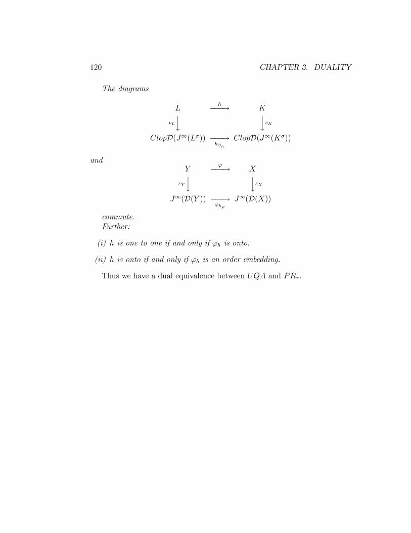
120 CHAPTER 3. DUALITY
The diagrams
Lh−−−→ K
vL
y yvK
ClopD(J∞(Lσ)) −−−→hϕh
ClopD(J∞(Kσ))
andY
ϕ−−−→ X
εY
y yεX
J∞(D(Y )) −−−→ϕhϕ
J∞(D(X))
commute.Further:
(i) h is one to one if and only if ϕh is onto.
(ii) h is onto if and only if ϕh is an order embedding.
Thus we have a dual equivalence between UQA and PRτ .

Chapter 4
A duality for SDMAs
4.1 Canonicity
We can apply the Sahlqvist Theory and canonicity of UQAs to the study ofsemi-De Morgan algebras and some of its subvarieties.
In fact, it is possible to identify SDMAs with algebras (L,∧,∨,B, 0, 1)where the unary operation is B=′ subjected to the additional restrictions
1. B 1 ≤ 0
2. BB a∧ BB b ≤BB (a ∧ b).
3. BBB a ≤B a and B a ≤BBB a.
It is clear that, by the definition of B (Definition 3.1.24 (iii)), this setof inequalities characterizes SDMA because the dual of condition 2 is aconsequence of BB being order preserving.
However not all these inequalities are Sahlqvist (Definition 3.1.33).We are going to show that BB a∧ BB b ≤BB (a∧b) is neither 1-Sahlqvist
nor ∂-Sahlqvist.The generation trees for these terms are respectively:
(+) a bc.n (−) B b
bu.n (+) B
b ∧(+)
b (+)bB (−) c.nb
JJ
J b B (+) u.n
(−) a b
b ∧(−) c.nJ
JJb b (−)
b B (+) u.n
b B (−) c.n
121

122 CHAPTER 4. A DUALITY FOR SDMAS
The term BB a∧ BB b is not 1-left Sahlqvist and it is ∂-left Sahlqvist.For 1-left Sahlqvist we have to worry about the positive occurrences of the
variables a and b. On the paths from these occurrences to the root we havethe prohibited configurations: we meet a choice node and then afterwards auniversal node as we travel from the variable up to the root. This is why thisterm is not 1-left Sahlqvist.
For ∂-left Sahlqvist, we have only to worry about the negative occurrencesof a and b. There aren’t any and thus the term is ∂-left Sahlqvist.
The term BB (a∧b) is 1-right Sahlqvist because in the negative generationtree there are no occurrences of a or b with (+) but it is not ∂-right Sahlqvistbecause there is a prohibited configuration in the paths of occurrences of aand b with (-).
Therefore the inequality is not Sahlqvist.
In [21] Theorem 3.7, M. Gehrke, H. Nagashi and Y. Venema prove thatthe first order formulas corresponding to Sahlqvist sequents can be effectivelycomputed. The theorem that is referred to yields the following:
Theorem 4.1.1. Every Sahlqvist inequality in a UQA+ corresponds to aformula in the first order language of the dual relational structure. This firstorder formula can be effectively computed from the inequality.
From the previous theorem it follows that Sahlqvist inequalities are par-ticularly useful. This is not the case of 2 so, it is advantageous for nicercorrespondence results (and thus duality) to consider a term-equivalent de-scription of SDMAs which casts them as UQAs with basic operations B=′
and 2 =′′. Accordingly we define:
Definition 4.1.2. Let SDMA be the class of algebras (L,∧,∨,B,2, 0, 1)satisfying
(M1) (L,∧,∨, 0, 1) ∈ DL
(M2) B 1 ≤ 0.
(M3) 2a ≤BB a.
(M4) BB a ≤ 2a.
(M5) B a ≤ 2 B a.

4.1. CANONICITY 123
(M6) 2 B a ≤B a.
All the inequalities M2,...,M6 are Sahlqvist (see Appendix). This is ratherinteresting because comparing this set of conditions with 1, 2 and 3 we con-clude that Sahlqvistness is not preserved under term equivalence.
For any (L,∧,∨,B,2, 0, 1) ∈ SDMA there is, as in UQA, a naturalembedding from this algebra in (Lσ,∧,∨,Bσ,2σ, 0, 1).
From Theorem 3.1.34 it follows that the inequalities M2,...,M6 are canon-ical so, if they are true in L, they are also true in Lσ. This means that thevariety SDMA is canonical and consequently (L,∧,∨,B,2, 0, 1) ∈ SDMAimplies (Lσ,∧,∨,Bσ,2σ, 0, 1) is what we might call a SDMA+, i.e. theintersection of SDMA with UQA+.
So we can define the following class of algebras.
Definition 4.1.3. Let SDMA+ be the class of algebras
(L,∧,∨, 0, 1,B,2) ∈ SDMA
such that L ∈ DL+ and, for any subset {ai : i ∈ I}
1. B 0 = 1 and B(∨
i∈I ai
)=∧
i∈I B ai.
2. 21 = 1 and 2(∧
i∈I ai
)=∧
i∈I 2ai.
Since SDMA is canonical, we have:
Theorem 4.1.4. If L ∈ SDMA then Lσ ∈ SDMA+.
In a similar way we can state that any subvariety of SDMA defined bySahlqvist inequalities is canonical. It is easy to characterize some importantsubvarieties of SDMA using conditions on 2 and B. In fact from Section1.4 (Remark 1.4.6, Remark 1.4.2, Definition 1.4.4 and Lemma 1.4.5), respec-tively, it follows:
Lemma 4.1.5. Let (L,∧,∨,B,2, 0, 1) ∈ SDMA. Then:
(i) L is in K1,1 if and only if B (a ∧ b) ≤B a∨ B b for any a, b ∈ L.
(ii) L is a De Morgan algebra if and only if 2a ≤ a and a ≤ 2a for eacha ∈ L.

124 CHAPTER 4. A DUALITY FOR SDMAS
(iii) L is a demi p-lattice if and only if B a ∧2a ≤ 0 for each a ∈ L.
(iv) L is an almost p-lattice if and only if B a ∧ a ≤ 0 for each a ∈ L.
(v) L is a p-lattice if and only if L is a demi p-lattice and a ≤ 2a for eacha ∈ L.
(vi) L is in the variety C if and only if for any a, b ∈ L inequalities γ andβ hold:
(γ) B (a ∧ b) ∧2b ≤B a∨ B b
(β) B (a ∧ b) ≤B a∨ B (B a ∧ b∧ B b)
Remark 4.1.6. It is now a simple exercise to verify that all these inequalitiesare Sahlqvist (see Appendix) and therefore they are all canonical.
4.1.1 Discrete Correspondence
Based on the duality established in Section 3.2 between UQA+ and PR weare going to determine the structures corresponding to SDMA+s.
For an algebra L ∈ SDMA+ (Definition 4.1.3), the dual structure is arelational structure (J∞(L),≤, RB, R2) where the relations RB and R2 haveto satisfy conditions corresponding to (M2),...(M6).
We have already proved that all these inequations are Sahlqvist so as aconsequence of Theorem 4.1.1 we know that we can effectively compute thecorresponding conditions:
For M2 we have:
B 1 ≤ 0⇔ ∀p ∈ J∞(L) : p 6≤B 1
⇔ ∀p ∈ J∞(L) ∃q ∈ J∞(L) : (q ≤ 1 and pRBq) by Lemma 3.2.9(i)
⇔ ∀p ∈ J∞(L) ∃q ∈ J∞(L) : pRBq
or equivalently,R−1
B (J∞(L)) = J∞(L)
For M3 we have:
∀a ∈ L : 2a ≤BB a if and only if
∀a ∈ L ∀p ∈ J∞(L) : (p ≤ 2a⇒ p ≤BB a)

4.1. CANONICITY 125
because L is join generated by J∞(L).Our objective now is to eliminate the universal quantifier in L, but first
observe that, by Lemma 3.2.9(iv), the previous condition is equivalent to:
∀a ∈ L∀p ∈ J∞(L) :(∨
(pR2) ≤ a⇒ p ≤BB a).
Notice that, given p, there is a least a for which the antecedent holds,namely a =
∨(pR2).
Also notice that if the conclusion holds for some a ∈ L then it holds forall greater a. Thus we get:
∀p ∈ J∞(L)(p ≤BB
(∨(pR2)
)). (4.1.1)
Now, by Lemma 3.2.9(ii):
p ≤BB(∨
(pR2))⇔ ∀q ∈ J∞(L)
(pRBq ⇒ q 6≤B
(∨(pR2)
))and, by Lemma 3.2.9(i):
q 6≤B(∨
(pR2))⇔ ∃r ∈ J∞(L)(r ≤
∨(pR2) and qRBr).
Since r ∈ J∞(L) and pR2 is a downset, we have r ≤∨
(pR2) if and onlyif pR2r.
Consequently, condition 4.1.1 is equivalent to
∀p, q ∈ J∞(L) (pRBq ⇒ ∃r ∈ J∞(L)(pR2r and qRBr))
so that M3 holds in L if and only if
RB ⊆ R2 ◦R∂B
For M4, observe that, since L is meet generated by M∞(L) = κ(J∞(L))(Theorem 3.1.7), BB a ≤ 2a holds in L if and only if
∀a ∈ L ∀p ∈ J∞(L)(κ(p) ≥ 2a⇒ κ(p) ≥BB a).
So we get, from Lemma 3.2.9 (iii):
∀a ∈ L ∀p ∈ J∞(L) ((∃q ∈ J∞(L)(pR2q and q 6≤ a))⇒ κ(p) ≥BB a)

126 CHAPTER 4. A DUALITY FOR SDMAS
or equivalently
∀a ∈ L ∀p, q ∈ J∞(L)((pR2q and κ(q) ≥ a)⇒ κ(p) ≥BB a).
Given p, q ∈ J∞(L) , notice that the greatest a ∈ L for which κ(q) ≥ aholds is a = κ(q) and if the conclusion holds for some a it also holds for allsmaller elements because BB is order preserving. Thus we get
∀p, q ∈ J∞(L)((pR2q ⇒ κ(p) ≥BB κ(q)).
Now, by Lemma 3.2.9 (i) and (ii) and by Remark 3.1.8, respectively, weobtain:
κ(p) ≥BB κ(q)⇔ ∃t ∈ J∞(L) (pRBt and t ≤B κ(q)))
⇔ ∃t ∈ J∞(L) (pRBt and (∀s ∈ J∞(L) (tRBs⇒ s 6≤ κ(q)))
⇔ ∃t ∈ J∞(L) (pRBt and (∀s ∈ J∞(L) (tRBs⇒ s ≥ q)) .
So M4 holds in L if and only if
∀p, q ∈ J∞(L) (pR2q ⇒ (∃t ∈ J∞(L) (pRBt and ∀s ∈ J∞(L)(tRBs⇒ s ≥ q))) .
For M5, B a ≤ 2 B a holds in L if and only if
∀a ∈ L ∀p ∈ J∞(L)(κ(p) ≥ 2 B a⇒ κ(p) ≥B a)
because L is meet generated by M∞(L).But, by Lemma 3.2.9 (iii) and (i):
κ(p) ≥ 2 B a
⇔ ∃q ∈ J∞(L) (pR2q and q 6≤B a)
⇔ ∃q ∈ J∞(L) (pR2q and (∃r ∈ J∞(L) (qRBr and r ≤ a))
⇔ ∃q, r ∈ J∞(L) (pR2q and qRBr and r ≤ a)
⇔ ∃r ∈ J∞(L) (pR2 ◦RBr and r ≤ a)
So we get,
∀a ∈ L∀p ∈ J∞(L) ((∃r ∈ J∞(L) (pR2 ◦RBr and r ≤ a))⇒ κ(p) ≥B a)
which is equivalent to
∀a ∈ L∀p, r ∈ J∞(L) ((pR2 ◦RBr and r ≤ a)⇒ κ(p) ≥B a)

4.1. CANONICITY 127
Given p, r ∈ J∞(L), the least a satisfying the antecedent is a = r, and ifthe conclusion holds for some a it holds for all greater values because B isorder reversing. Thus we get
∀p, r ∈ J∞(L) ((pR2 ◦RBr)⇒ κ(p) ≥B r)
That is, by the definition of RB(equation (3.2.3)),
∀p, r ∈ J∞(L) (p(R2 ◦RB)r ⇒ pRBr)
which is equivalent to
R2 ◦RB ⊆ RB
For M6, 2 B a ≤B a holds in L is equivalent to
∀a ∈ L ∀p ∈ J∞(L) (κ(p) ≥B a⇒ κ(p) ≥ 2 B a).
By Lemma 3.2.9 (i), this is equivalent to
∀a ∈ L∀p ∈ J∞(L)((∃q ∈ J∞(L)(pRBq and q ≤ a))⇒ κ(p) ≥ 2 B a)
and to
∀a ∈ L∀p, q ∈ J∞(L)((pRBq and q ≤ a)⇒ κ(p) ≥ 2 B a)
Given p, q ∈ J∞(L), the least a satisfying the antecedent is a = q and ifthe conclusion holds for some a it also holds for all greater elements, so weget
∀p, q ∈ J∞(L) (pRBq ⇒ κ(p) ≥ 2 B q)
Now
κ(p) ≥ 2 B q ⇔ ∃r ∈ J∞(L) (pR2r and r 6≤B q) by Lemma 3.2.9(iii)
⇔ ∃r ∈ J∞(L) (pR2r and rRBq) by the definition of RB
⇔ pR2 ◦RBq
That is, M6 holds in L if and only if
∀p, q ∈ J∞(L)(pRBq ⇒ pR2 ◦RBq)

128 CHAPTER 4. A DUALITY FOR SDMAS
or equivalentlyRB ⊆ R2 ◦RB.
Notice that in all the previous proofs the correspondence between Sahlqvistequations and conditions in RB and R2 was always obtained using the strat-egy of eliminating the universal quantifier on elements of L.
It is now possible to define the dual structures of SDMA+s. We willdenote by PRM these structures:
Definition 4.1.7. Let PRM be the class of relational structures (X,≤, R2, RB) where (X,≤) is a partially ordered set and R2, RB are binary re-lations on X such that:
(F1) ≥ ◦R2◦ ≥= R2
(F2) ≥ ◦RB◦ ≤= RB
(F3) R−1B (X) = X
(F4) RB ⊆ R2 ◦R∂B
(F5) ∀p, q ∈ X (pR2q ⇒ ∃t ∈ X (pRBt and ∀s ∈ X(tRBs⇒ s ≥ q)) .
(F6) RB = R2 ◦RB
Since we have proved the equivalence of conditions M2,...,M6 and F3,...,F6it is possible to define a map ()+ : SDMA+ → PRM . On the other hand,when we have a relational structure, (X,≤, R2, RB) ∈ PRM it is easy toprove that (D(X),∩,∪, ∅, X,2R,BR) is in SDMA+.
So we conclude, applying Theorem 3.2.8,
Theorem 4.1.8. There exist maps
()+ : SDMA+ −→ PRM and ()+ : PRM −→ SDMA+
such that for each L ∈ SDMA+ and each X ∈ PRM ,
(L)+ = (J∞(L),≤, R2, RB) and (X)+ = (D(X),∪,∩, ∅, X,2R,BR).
The function ηL : L −→ ((L)+)+ is a complete isomorphism and thefunction εX : X −→ ((X)+)+ is an isomorphism for the relations ≤, R2 andRB.

4.1. CANONICITY 129
Naturally, morphisms in SDMA+ are complete {0,1}-homomorphismsand morphisms in PRM are order preserving maps satisfying conditions (ii)and (iii) from definition 3.2.11 so that we can establish as in Theorem 3.2.12a correspondence between these morphisms.
This way we obtain a dual equivalence between SDMA+ and PRM .
We are going to see that the conditions defining morphisms in PRM arenot independent:
Theorem 4.1.9. Let X, Y be relational structures in PRM and let ϕ : X →Y be an order preserving map. Then ϕ ∈ PRM(X, Y ) if and only if thefollowing conditions hold:
(a) ∀q, r ∈ X : (qRBr ⇒ ϕ(q)RBϕ(r)) .
(b) ∀q ∈ X ∀p ∈ Y : (ϕ(q)RBp⇒ (∃r ∈ X : (ϕ(r) ≤ p and qRBr)).
Proof. We have only to prove that (a) and (b) imply conditions (ii) fromdefinition 3.2.11.
For the first implication of (ii) we have, for any q, r ∈ X,
qR2r ⇒⇒ ∃t ∈ X (qRBt and (∀s ∈ X (tRBs⇒ s ≥ r))) by F5
⇒ ∃t ∈ X (ϕ(q)RBϕ(t) and (∀s ∈ X (tRBs⇒ s ≥ r))) by (a)
⇒ ∃t ∈ X∃u ∈ Y (ϕ(q)R2u and ϕ(t)RBu and (∀s ∈ X (tRBs⇒ s ≥ r))) by F4
⇒ ∃t ∈ X∃u ∈ Y (ϕ(q)R2u and ∃v ∈ X (ϕ(v) ≤ u and tRBv) and
and (∀s ∈ X (tRBs⇒ s ≥ r)) by (b) .
From here it follows,
∃t, v ∈ X (ϕ(q)R2◦ ≥ ϕ(v) and v ≥ r)) .
By F1 and since ϕ is order preserving we have
∃v ∈ X (ϕ(q)R2ϕ(v) and ϕ(v) ≥ ϕ(r))
and, again by F1,ϕ(q)R2ϕ(r).
In what concerns the second implication of (ii):

130 CHAPTER 4. A DUALITY FOR SDMAS
For every q ∈ X and p ∈ Y ,
ϕ(q)R2p⇒⇒ ∃r ∈ Y (ϕ(q)RBr and (∀s ∈ Y rRBs⇒ s ≥ p)) by F5
⇒ ∃r ∈ Y ∃t ∈ X (ϕ(t) ≤ r and qRBt and (∀s ∈ Y (rRBs⇒ s ≥ p))) by (b)
⇒ ∃r ∈ Y ∃t, u ∈ X (ϕ(t) ≤ r and qR2u and tRBu and (∀s ∈ Y (rRBs⇒ s ≥ p)))
by F4
⇒ ∃r ∈ Y ∃t, u ∈ X (r ≥ ϕ(t) and ϕ(t)RBϕ(u) and qR2u and
(∀s ∈ Y (rRBs⇒ s ≥ p))) because ϕ is order preserving
⇒ ∃r ∈ Y ∃u ∈ X (r ≥ ◦RBϕ(u) and qR2u and (∀s ∈ Y (rRBs⇒ s ≥ p)))
As a consequence of F1 we have
∃r ∈ Y ∃u ∈ X (rRBϕ(u) and (∀s ∈ Y : rRBs⇒ s ≥ p) and qR2u)
and finally we obtain
∃u ∈ X (ϕ(u) ≥ p and qR2u).
This way we can define morphisms in PRM as order preserving mapssatisfying conditions (a) and (b) of the previous theorem.
In order to simplify the duality we have obtained for SDMA+, we aregoing to prove some other properties that are true in PRM .
First observe that, from F4, it follows that
R∂B ⊆ RB ◦R∂
2
so, again by F4,RB ⊆ R2 ◦RB ◦R∂
2.
Finally, by F6 ,
(F7) RB ⊆ RB ◦R∂2.
Now we are going to study those elements of X ∈ PRM that are maximalin pR2 or minimal in pRB for some p ∈ X. For these elements we have:

4.1. CANONICITY 131
Lemma 4.1.10. Let X ∈ PRM and let p, q ∈ X be such that q is a maximalelement of pR2. Then there is t ∈ X such that pRBt and q is the minimumof tRB.
Proof. From F5, we know that pR2q implies:
∃t ∈ X (pRBt and (∀u ∈ X (tRBu⇒ u ≥ q)).
But, by F4, it follows from pRBt that there is v ∈ X such that pR2v and tRBv.Therefore v ≥ q.
Since q is maximal in pR2 we must have v = q.Then we conclude that q is the minimum of tRB because we have tRBq
and ∀u ∈ X, (tRBu⇒ u ≥ q).
Lemma 4.1.11. Let X ∈ PRM and let p, q ∈ X be such that q is a minimalelement of pRB. Then there is t ∈ X such that pRBt and q is the maximumof tR2
Proof. Since we have pRBq we know, by F6, that
∃r ∈ X(pR2r and rRBq)
and, from F5 and pR2r,
∃t ∈ X (pRBt and ∀u ∈ X : (tRBu⇒ u ≥ r)) . (∗)
Now, for any s ∈ X such that tR2s, we have, by F5, that t is such that
∃y ∈ X(tRBy and ∀w ∈ X(yRBw ⇒ w ≥ s)). (∗∗)
By condition (∗), tRBy implies y ≥ r and, since rRBq, we have, by F2,yRBq. Therefore, by (∗∗), q ≥ s.
So we proved that t and q are such that
∀s ∈ X(tR2s⇒ q ≥ s). (∗ ∗ ∗)
From pRBt and F7 it follows that there is z ∈ X such that pRBz andtR2z.
So we have q ≥ z by condition (∗ ∗ ∗) and, since q is minimal in pRB, wehave z = q and hence tR2q.
By (∗ ∗ ∗), we conclude that q is the maximum of tR2.

132 CHAPTER 4. A DUALITY FOR SDMAS
Now we can define
Definition 4.1.12. Let X ∈ PRM . We will denote by W the subset
W = {q ∈ X : ∃p ∈ X q is minimal in pRB}
It is clear from Lemmas 4.1.10 and 4.1.11 that the following holds:
W = {q ∈ X : ∃p ∈ X q is maximal in pR2}. (4.1.2)
It is possible to obtain another characterization of W :
Lemma 4.1.13. Let X ∈ PRM and let q ∈ X. Then q ∈ W if and only if
qR2q and ∀r ∈ X(qRBr ⇒ rRBq).
Proof. (⇐) Let q ∈ X be such that qR2q and ∀r ∈ X(qRBr ⇒ rRBq).Since we have qR2q then, by F5, there is t ∈ X such that
qRBt and ∀s ∈ X (tRBs⇒ s ≥ q).
Then we have also tRBq, so we conclude that q is the minimum of tRB
and thus, q ∈ W .(⇒)Let q ∈ W . Then, there is p ∈ X such that pR2q and q is maximal in
pR2 by condition (4.1.2).By Lemma 4.1.10 there is s ∈ X such that q is the minimum of sRB.From F7 and sRBq it follows that there is u ∈ X such that sRBu and
qR2u so, since q is the minimum of sRB, we have u ≥ q and, by F2, qR2q.Since q is minimal in sRB there is t ∈ X such that q is the maximum of
tR2.Now, for any r ∈ X, qRBr implies tRBr by F6 and, from F4 it follows
that there is v ∈ X such that tR2v and rRBv so v ≤ q because q is themaximum of tR2 and, by F1, rRBq.
In order to obtain a simpler duality for SDMAs we will use the binaryrelation Rmin
B that we considered in Section 3.3. For practical reasons we willdenote this relation by S.
4.2. CORRESPONDENCE FOR CANONICAL EXTENSIONS 133
Definition 4.1.14. Let X ∈ PRM and let p, q ∈ X. We call S the binaryrelation such that
pSq if and only if pRBq and q is minimal in pRB
From Definition 4.1.12 it follows that
W = Im(S).
It is obvious, for those familiar with Hobby’s duality for SDMAs [25]that this relation S is the correspondent of the binary relation ← defined byD. Hobby in the poset of prime ideals of a SDMA.
4.2 Correspondence for canonical extensions
The relation S ⊆ X × X becomes particularly interesting when there is asemi-De Morgan algebra L such that X = J∞(Lσ) where Lσ is the canonicalextension of L. In fact, when this happens we can apply Theorem 3.3.2 (ii)and, from Definition 4.1.7 (F3) and Definition 4.1.12, we conclude:
Lemma 4.2.1. Let Lσ ∈ SDMA+ be the canonical extension of L ∈ SDMAand let X = J∞(Lσ). Then
S−1(X) = S−1(W ) = X.
When we consider the restriction of S to the subset W we have:
Lemma 4.2.2. Let L ∈ SDMA and X = J∞(Lσ). Then, S ∩ (W ×W ) isan order reversing involution.
Proof. We have to prove that S is such that:
(i) For any q ∈ W there is one and only one element r ∈ W such that qSrand, for this element r we have also rSq.
(ii) For any p, q, r, u ∈ W such that qSr and pSu, if q ≥ p then u ≥ r.
To prove (i) note that for every q ∈ W we have qR2q so, according to F5,
∃t ∈ X (qRBt and ∀s ∈ X(tRBs⇒ s ≥ q)). (∗)

134 CHAPTER 4. A DUALITY FOR SDMAS
From Theorem 3.3.2, we know that there is r ∈ W such that r is aminimal element of qRB and r ≤ t. Therefore r is such that qSr.
By Lemma 4.1.13, we have also rRBq.On the other hand, by F2, we know that for any s ∈ X, rRBs implies
tRBs because t ≥ r.It follows from (∗) that
∀s ∈ X (rRBs⇒ s ≥ q)
so q is the minimum of rRB and hence rSq.In an analogous way, from r ∈ W and rR2r it follows that there is x ∈ W
such that rSx and xSr and r is the minimum of xRB. But we know that qis the minimum of rRB so we have q = x and, since both sets qRB and rRB
have minimums, these elements are unique.To prove (ii) notice that, by F2, q ≥ pSu implies qRBu. Since r is the
minimum of qRB we obtain u ≥ r.
From the previous Lemma it follows that, for any p ∈ W , the set pRB
has a minimum and that
∀p, q ∈ W, pS2q ⇔ p = q.
It is clear how Lemma 4.2.2 generalizes the dual description of De MorganAlgebras obtained by Cornish and Fowler in [14]. In fact, when X = W , thespace X is the dual of a De Morgan Algebra and the relation S correspondsto the involution ξ of Cornish and Fowler’s duality.
We have already studied the relation S2 in W ×W . When we considerthe relation S2 ⊆ X ×X we have:
Lemma 4.2.3. Let X = J∞(Lσ) with L ∈ SDMA. Then, for any p, q ∈ X,we have
pS2q if and only if q is maximal in pR2.
Proof. (⇐)Suppose that q is maximal in pR2q. Then q ∈ W so, by Lemma 4.2.2,
there is one and only one r ∈ W such that qSr and, by F6, pRBr.By Theorem 3.3.2 there is t ∈ W such that t ≤ r and pSt and, by Lemma
4.2.2, there is u ∈ W such that tSu and uSt.

4.2. CORRESPONDENCE FOR CANONICAL EXTENSIONS 135
Since S is an involution in W , t ≤ r implies q ≤ u.On the other hand, from pSt it follows, by F4, that there is v ∈ X such
that pR2v and tRBv. But t ∈ W so u is the minimum of tRB and henceu ≤ v.
So we have q ≤ u ≤ v and pR2v. Since q is maximal in pR2, q = u = vand consequently pStSq.
(⇒)For the converse suppose that p, q are such that pS2q. Then q ∈ W and
there is u ∈ W such that pSu and uSq.From F4 and pSu, there is x ∈ X such that pR2x and uRBx. But
u, q ∈ W so, x ≥ q because q is the minimum of uRB. From F1 it followsthat pR2q.
By Theorem 3.3.2 there is w ∈ W such that w ≥ q and w is maximal inpR2.
As a consequence of the if part, pS2w holds so that there is z ∈ W suchthat pSz and zSw.
But then we get zSw, uSq and w ≥ q with all these elements in W . Itfollows from Lemma 4.2.2 that z ≤ u. Since we have simultaneously pSuand pSz we conclude that z = u and consequently q = w.
So, q is maximal in pR2.
From the previous Lemmas we conclude the following theorem that char-acterizes the relation S:
Theorem 4.2.4. Let L ∈ SDMA and let X = J∞(Lσ) ∈ PRM . Then thebinary relation S ⊆ X ×X has the following properties:
(H1) ≥ ◦S ⊆ S◦ ≤.
(H2) Dom(S) = {p ∈ X : ∃q ∈ X pSq} = X.
(H3) For each p ∈ X, pS is an antichain.
(H4) On W = {q ∈ X : ∃p ∈ X pSq}, S is an involution.
Proof. It is clear that (H1) follows from F1 and Theorem 3.3.2 and that (H2)is a direct consequence of Lemma 4.2.1.
The definition of S implies (H3) and condition (H4) follows from Lemma4.2.2.

136 CHAPTER 4. A DUALITY FOR SDMAS
Now we can think of a relational structure (X,≤, S) where X = J∞(Lσ)for some L ∈ SDMA and S satisfies conditions H1,...,H4. We will denotethese structures by PRS.
We can prove the following:
Theorem 4.2.5. Let (X,≤, S) ∈ PRS and let
RB = S◦ ≤ and R2 = S2◦ ≥ .
Then (X,≤, R2, RB) ∈ PRM and, for any U ∈ D(X),
R−1B (U) = S−1(U) and R−1
2 (U) = S−1(X \ S−1(U)).
Proof. From the definition of RB it is obvious that F2 follows from H1 whileF3 is a direct consequence of H2.
In what concerns F1 notice that, for any p, q ∈ X,
p ≥ ◦R2◦ ≥ q ⇔ p ≥ ◦S2◦ ≥ q ⇔ ∃y, z ∈ W, p ≥ ◦SySz ≥ q.
By H1 this implies
∃y, z ∈ W, pS◦ ≤ ySz ≥ q ⇔ ∃x, y, z ∈ W, pSx ≤ ySz ≥ q.
Since x, y, z ∈ W , it follows from H4 that there is t ∈ W such that t ≥ z andxSt and hence we obtain:
pSxSt ≥ q ⇔ pS2◦ ≥ q ⇔ pR2q.
For F4 observe that from the definition of RB and H4,
pRBq ⇔ ∃x ∈ W, pSx ≤ q ⇔ ∃x, y ∈ W, pSxSySx ≤ q.
But this implies pS2y and q ≥ xSy or, by H1, qS◦ ≤ y and consequentlypR2y and qRBy.
To prove F5:
pR2q ⇔ pS2◦ ≥ q ⇔ ∃x, y ∈ W, pSxSy ≥ q.
This implies pRBx and since x ∈ W ,
∀s ∈ X, xRBs⇒ xSy ≤ s⇒ s ≥ y ≥ q.

4.2. CORRESPONDENCE FOR CANONICAL EXTENSIONS 137
For F6, observe that on one side we have, by the definition of RB and H4:
pRBq ⇔ ∃x ∈ W, pSx ≤ q ⇔ ∃x, y ∈ W, pSxSySx ≤ q
from here it follows that pS2y and yS◦ ≤ q. Consequently pR2y and yRBq.For the converse we have, by H1 and H4 respectively, that for any y ∈ X:
pR2y and yRBq ⇔ pS2◦ ≥ yS◦ ≤ q ⇒ pS3◦ ≤ q ⇒ pS◦ ≤ q ⇔ pRBq.
So we proved that (X,≤, R2, RB) ∈ PRM .Now, to prove that R−1
B (U) = S−1(U) for any U ∈ D(X), observe thatthe inclusion R−1
B (U) ⊇ S−1(U) is evident.For the other inclusion notice that, for any p ∈ R−1
B (U) there is q ∈ Usuch that pRBq and, by the definition of RB, pS◦ ≤ q so, there is t ∈ X suchthat t ≤ q and pSt. But U is a downset so t ∈ U and thus p ∈ S−1(U).
For the proof of the second equation suppose that p ∈ X is such thatp ∈ S−1(X \ S−1(U)).
Then there is q 6∈ S−1(U) such that pSq. By H4, there is one and only oneelement r ∈ W such that qSr. It is clear now that r ∈ X \U and, since pS2rwe have pR2r so that p ∈ R−1
2 (X \U). Thus R−12 (X \U) ⊇ S−1(X \S−1(U)).
Now let p ∈ R−12 (X \ U). Then there is q 6∈ U such that pR2q or, by the
definition of R2, pS2◦ ≥ q.Hence there are y, t ∈ W such that pSySt ≥ q. Since U is a downset and
q 6∈ U we have also t 6∈ U and, since t is the only element such that ySt,y ∈ X \ S−1(U). Therefore p ∈ S−1(X \ S−1(U)).
Consequently R−12 (X \ U) ⊆ S−1(X \ S−1(U)).
From the previous theorems we conclude that there is an alternative du-ality between the class of structures (X,≤, S) ∈ PRS and SDMA+.
From Theorem 4.2.5, it is obvious that we can define the unary operationsin D(X) by
B (U) = X \ S−1(U) and 2(U) = X \ (S−1(X \ S−1(U)) (4.2.1)
for any U ∈ D(X).
Now we are going to study morphisms between structures (X,≤, S) and(Y,≤, S) in PRS:
138 CHAPTER 4. A DUALITY FOR SDMAS
Theorem 4.2.6. Let L,K ∈ SDMA and let X = J∞(Lσ) and Y = J∞(Kσ)and ϕ : X → Y be an order preserving map. Then ϕ ∈ PRM(X, Y ) if andonly if
(c) ∀q ∈ X∀p ∈ Y, (ϕ(q)S◦ ≤ p⇔ (∃r ∈ X, ϕ(r) ≤ p and qSr)).
Proof. First suppose that ϕ ∈ PRM(X, Y ) so that the conditions (a) and(b) in Theorem 4.1.9 hold.
(⇒)Let q ∈ X and p ∈ Y be such that ϕ(q)S◦ ≤ p. Then ϕ(q)RBp and from
(b),∃t ∈ X (ϕ(t) ≤ p and qRBt).
So, by the definition of RB,
∃r, t ∈ X (ϕ(t) ≤ p and qSr and r ≤ t)
and, since ϕ is order preserving,
∃r ∈ X (ϕ(r) ≤ p and qSr).
(⇐)Now suppose that q ∈ X and p ∈ Y and that there is r ∈ X such that
ϕ(r) ≤ p and qSr.By the definition of RB, ϕ(r) ≤ p and qRBr so, by condition (a),
ϕ(r) ≤ p and ϕ(q)RBϕ(r).
Thus ϕ(q)RB◦ ≤ p and consequently ϕ(q) ≥ ◦S◦ ≤ p. By H1 we concludethat ϕ(q)S◦ ≤ p.
For the converse observe that condition (b) is a direct consequence of thedefinition of S and condition (c).
For condition (a), notice that if qRBr then there is x ≤ r such that qSxand, since ϕ is an order preserving map ϕ(x) ≤ ϕ(r). So, by condition (c),ϕ(q)S◦ ≤ ϕ(r) and, consequently, ϕ(q)RBϕ(r).
Thus we have the following
Definition 4.2.7. Let X,Y ∈ PRS and let ϕ : X → Y be an order preserv-ing map. We say that ϕ ∈ PRS(X, Y ) if and only if
(c) ∀q ∈ X∀p ∈ Y, (ϕ(q)S◦ ≤ p⇔ (∃r ∈ X, ϕ(r) ≤ p and qSr)).

4.2. CORRESPONDENCE FOR CANONICAL EXTENSIONS 139
Observe that if, for any p ∈ X, we consider the subset pS = {q ∈ X : pSq}then condition (c) is equivalent to the simpler equality
↑ (ϕ(q)S) =↑ ϕ(qS)
for any q ∈ X. This shows how ϕ(q)S and ϕ(qS) generate the same upset.
Since the ranges of morphisms play an important role in the study ofcongruences, notice that, as in Corollary 3.3.3, we have also:
Corollary 4.2.8. Let X = J∞(Lσ) and Y = J∞(Kσ) where J∞(Lσ) andJ∞(Kσ) are the canonical extensions of L,K ∈ SDMA. Let ϕ : X → Y bea morphism in PRS.
Then ϕ(X) is closed for the relation S.

140 CHAPTER 4. A DUALITY FOR SDMAS
4.2.1 Topological duality for SDMAs
As an application of the duality we have established for UQAs we are goingto present a duality for semi-De Morgan Algebras.
We will identify the variety of SDMAs with the class of algebras (L,∧,∨,B,2, 0, 1) from Definition 4.1.2 as we have been doing in the previous sections.
Since the variety SDMA is canonical we will consider the natural embed-ding of an SDMA (L,∧,∨, 0, 1,B,2) in (Lσ,∧,∨, 0, 1,Bσ,2σ) ∈ SDMA+
(Theorem 4.1.4).
We have already established, in section 4.1.1, Theorems 4.1.8 and 4.1.9,a duality between perfect SDMA+ and the relational structures PRM .
To find the dual spaces of SDMAs we have to consider, as in UQA,a topology in the relational space. Therefore, we will define the followingrelational structures:
Definition 4.2.9. Let PRM τ be the class of relational structures (X,≤, τ, R2, RB) where (X,≤, τ) is a Priestley space and R2, RB are binary rela-tions on X such that:
(F1) (i) ≥ ◦R2◦ ≥= R2.
(ii) For each U ∈ ClopD(X), X \R−12 (X \ U) ∈ ClopD(X).
(iii) For each p ∈ X, pR2 = {q ∈ X : pR2q} is closed.
(F2) (i) ≥ ◦RB◦ ≤= RB
(ii) For each U ∈ ClopD(X), X \R−1B (U) ∈ ClopD(X).
(iii) For each p ∈ X, pRB = {q ∈ X : pRBq} is closed.
(F3) R−1B (X) = X
(F4) RB ⊆ R2 ◦R∂B
(F5) ∀p, q ∈ X (pR2q ⇒ ∃t ∈ X (pRBt and ∀s ∈ X(tRBs⇒ s ≥ q)) .
(F6) RB = R2 ◦RB
We are going to prove:

4.2. CORRESPONDENCE FOR CANONICAL EXTENSIONS 141
Theorem 4.2.10. There exist maps
D : SDMA −→ PRM τ and E : PRM τ −→ SDMA.
such that the function ηL : L −→ E(D(L)) is an isomorphism and the func-tion εX : X −→ D(E(X)) is an order homeomorphism and an isomorphismfor the relations R2 and RB.
Proof. To define D notice that if L ∈ SDMA then, by Theorem 4.1.4, wehave Lσ ∈ SDMA+.
But for this class of algebras we have already a duality so, by Theorem4.1.8, (J∞(Lσ),≤, R2, RB) ∈ PRM and consequently conditions F1 (i), F2(i),F3, F4, F5 and F6 hold.
On the other hand we know by Theorem 3.4.22 that (J∞(Lσ),≤, τ, R2, RB)is a Priestley space where conditions F1 (i), (ii),(iii) and F2 (i), (ii), (iii) aresatisfied.
So we can take D(L) to be (J∞(Lσ),≤, τ, R2, RB) ∈ PRM τ
To define E, let us consider X ∈ PRM τ . Then we have also X ∈ PRMand by Theorem 4.1.8, (D(X),∩,∪, ∅, X,2R,BR) where
2R(U) = X \R−12 (X \ U) and BR (U) = X \R−1
B (U)
is in SDMA+.By Theorem 3.4.22 we can conclude that (ClopD(X),∩,∪, ∅, X,2R,BR)
is in SDMA. In fact if conditions (M2),...,(M6) from definition 4.1.2 hold inD(X) then they are also true in ClopD(X).
Thus we will define E(X) = (ClopD(X),∩,∪, ∅, X,2R,BR) ∈ SDMAThe properties of ηL and εX follow from Theorem 3.4.22.
Thus we have defined at the objects level a duality between SDMA andPRM τ .
To define functorsD and E between morphisms of these two categories ob-serve that morphisms in SDMA are {0,1}-homomorphisms while morphismsin PRM τ have to respect the topology so they are continuous order preserv-ing maps. On the other hand, since for every (X,≤, τ, R2, RB) ∈ PRMτ
we have also (X,≤, R2, RB) ∈ PRM , we will have by Theorem 4.1.9 thefollowing

142 CHAPTER 4. A DUALITY FOR SDMAS
Definition 4.2.11. Let X,Y be relational structures in PRM τ and letϕ : X → Y be a continuous order preserving map. Then we say ϕ ∈PRM τ (X, Y ) if and only if the following conditions hold:
(a) ∀q, r ∈ X : (qRBr ⇒ ϕ(q)RBϕ(r)) .
(b) ∀q ∈ X ∀p ∈ Y : (ϕ(q)RBp⇒ (∃r ∈ X : (ϕ(r) ≤ p and qRBr)).
We can prove:
Theorem 4.2.12. Let L,K ∈ SDMA and let X, Y ∈ PRM τ . Givena morphism h ∈ SDMA(L,K), there is an associated morphism ϕh ∈PRM τ (J∞(Kσ), J∞(Lσ)) defined by
ϕh(p) =∧{a ∈ L : p ≤ h(a)}
with all p ∈ J∞(Kσ).Given a morphism ϕ ∈ PRM τ (Y,X), there is an associated morphism
hϕ ∈ SDMA(ClopD(X), ClopD(Y )) defined by
hϕ = ϕ−1(U)
for each U ∈ ClopD(X).The maps D : SDMA(L,K) −→ PRM τ (J∞(Kσ), J∞(Lσ)) such that
D(h) = ϕh and E : PRM τ (Y,X) −→ SDMA(ClopD(X), ClopD(Y )) suchthat E(ϕ) = hϕ are bijections.
The diagrams
Lh−−−→ K
vL
y yvK
ClopD(J∞(Lσ)) −−−→hϕh
ClopD(J∞(Kσ))
andY
ϕ−−−→ X
εY
y yεX
J∞(D(Y )) −−−→ϕhϕ
J∞(D(X))
commute.Further:

4.2. CORRESPONDENCE FOR CANONICAL EXTENSIONS 143
(i) h is one to one if and only if ϕh is onto.
(ii) h is onto if and only if ϕh is an order embedding.
Proof. Let h ∈ SDMA(L,K) Then we have, since h is a {0,1}-homomor-phism that hσ ∈ SDMA+(Lσ, Kσ) and, as we saw in Theorem 4.2.12, ϕh ∈PRM . By Lemma 3.4.6, ϕh is continuous so ϕh ∈ PRM τ .
Let ϕ ∈ PRM τ (Y,X). Then ϕ ∈ Pτ (Y,X) and, from Lemma 3.4.7,it follows that hϕ such that hϕ = ϕ−1(U) for every U ∈ ClopD(X) is amorphism in DL(ClopD(X), ClopD(Y )).
On the other hand we have also ϕ ∈ PRM(Y,X) so there is a homomor-phism Hϕ ∈ SDMA+(D(X),D(Y )) such that for each V ∈ D(X) we haveHϕ(V ) = ϕ−1(V ) . Then hϕ = (Hϕ)�ClopD(X) so hϕ ∈ SDMA.
The other statements in the theorem are a consequence of Theorem 3.4.8
So we have established that the categories SDMA and PRM τ are duallyequivalent.
Naturally we will obtain a much simpler duality if we consider, as inSection 4.2, ordered structures with the relation S (Definition 4.1.14). Butnow we have also to bear in mind that there is a topology in the ordered space.Let us find out how S interacts with the topology τ in the new structures.
Definition 4.2.13. Let PRSτ be the class of relational structures (X,≤, τ, S) where (X,≤, τ) is a Priestley space and S is a binary relation on Xsuch that:
(H1) (i) ≥ ◦S ⊆ S◦ ≤ .
(ii) For each U ∈ ClopD(X), X \ S−1(U) ∈ ClopD(X).
(iii) For each p ∈ X, ↑ (pS) = {q ∈ X : pS◦ ≤ q} is closed.
(H2) Dom(S) = {p ∈ X : ∃q ∈ X pSq} = X.
(H3) For each p ∈ X, pS is an antichain.
(H4) On W = {q ∈ X : ∃p ∈ X pSq}, S is an involution.
Now we can prove:

144 CHAPTER 4. A DUALITY FOR SDMAS
Lemma 4.2.14. Let (X,≤, τ, R2, RB) ∈ PRM τ and let S = RminB . Then
(X,≤, τ, S) ∈ PRSτ .
Proof. We have already proved in Theorem 4.2.5 that R−1B (U) = S−1(U) for
every U ∈ D(X) and it is clear that ↑ (pS) = pRB by the definition of S soH1 (ii) and (iii) are verified.
The other conditions follow from Theorem 4.2.4.
Conversely
Lemma 4.2.15. Let (X,≤, τ, S) ∈ PRSτ and let RB = S◦ ≤ and R2 =S2◦ ≥. Then (X,≤, τ, R2, RB) ∈ PRM τ .
Proof. The equivalence between H2,..., H4 and F3,..., F6 was already verifiedin Theorems 4.2.4 and 4.2.5 and conditions F1 (i) and F2 (i) are a directconsequence of the way RB and R2 were defined there.
From Theorem 4.2.5 and H1 (ii), it is clear that conditions F1 (ii) and F2(ii) hold in X so we have just to prove that pR2 is closed.
To do so observe that pR2 =↓ pS2 by the definition of R2.Now, let q 6∈↓ pS2. Then for every r ∈ pS2, q 6≤ r. Since X is a Priestley
space there is a clopen downset Ur such that r ∈ Ur and q ∈ X \Ur. Clearly↓ pS2 ⊆
⋃r∈pS2 Ur.
By H1(ii), for each r ∈ pS2, S−1(Ur) is a clopen upset so, to prove that↑ pS ⊆
⋃r∈pS2 S−1(Ur), it is enough to see that pS ⊆
⋃r∈pS2 S−1(Ur).
Let r ∈ pS. Then r ∈ W and pSr so there is one and only one t ∈ Wsuch that pSrSt. Then t ∈ pS2 so that t ∈ Ut and consequently r ∈ S−1(Ut)so r ∈
⋃r∈pS2 S−1(Ur).
Now remember that ↑ pS is closed so that there is a finite number ofupsets S−1(Ur1), ..., S
−1(Urn) such that ↑ pS ⊆ S−1(Ur1)∪ ...∪S−1(Urn). Weare going to prove that ↓ pS2 ⊆ Ur1 ∪ ...Urn .
Let x ∈ pS2 then x ∈ W so, there is y ∈ W such that pSySx. Theny ∈↓ pS so, there is Urk
with 1 ≤ k ≤ n such that y ∈ S−1(Urk). Since
y ∈ W , x is the only element such that ySx so x ∈ Urk.
Therefore pS2 ⊆ Ur1 ∪ ...Urn and since ↓ pS2 is a downset, ↓ pS2 ⊆Ur1 ∪ ...Urn .
From here we conclude that X\Ur1∩...∩X\Urn , is an open neighborhoodof q that is disjoint from ↓ pS2. So, ↓ pS2 is closed.

4.2. CORRESPONDENCE FOR CANONICAL EXTENSIONS 145
It is now obvious that at the objects level we can establish a dualitybetween SDMA and PRSτ .
Regarding morphisms, Theorem 4.2.6 shows how to define such maps inorder that both categories PRM and PRSτ are equivalent. So we have:
Definition 4.2.16. Let L,K ∈ SDMA and let X = J∞(Lσ) and Y =J∞(Kσ) and ϕ : X → Y be a continuous order preserving map. Thenϕ ∈ PRSτ if and only if
(c) ∀q ∈ X∀p ∈ Y, (ϕ(q)S◦ ≤ p⇔ (∃r ∈ X, ϕ(r) ≤ p and qSr)).
Applying Theorem 4.2.10, Lemma 4.2.14 and Lemma 4.2.15 we can definedirectly the functors D and E between SDMA and PRSτ obtaining thefollowing:
Theorem 4.2.17. Let L ∈ SDMA and let D(L) = (J∞(Lσ),≤, τ, S) whereS is such that pSq if and only if q is a minimal element in {r ∈ J∞(Lσ) :κ(p) ≥B q}.
Let (X,≤, τ, S) ∈ PRSτ and let E(X) = (ClopD(X),∩,∪, ∅, X,B,2)where, for any U ∈ ClopD(X), B (U) = X \ S−1(U) and 2(U) = X \S−1(X \ S−1(U)).
Then D maps SDMA in PRSτ and E maps PRSτ in SDMA.Further, D and E define a dual equivalence between SDMA and PRSτ .
Clearly we obtained this way a category PRSτ that is dually equivalentto SDMA.
In this duality notice that the correspondents of congruences in SDMAsare closed subsets of the dual space that are closed for S. In fact, fromCorollary 3.4.9 it follows that, since any congruence θ of a semi-De Morganalgebra L is a congruence of the distributive lattice, there is a a closed subsetZ ⊆ J∞(Lσ) corresponding to θ and, for any a, b ∈ L:
aθb⇔ v(a) ∩ Z = v(b) ∩ Z
where v(a) = {p ∈ J∞(Lσ) : p ≤ a} and v(b) = {p ∈ J∞(Lσ) : p ≤ b}.Since the subset Z is the range of the morphism in PRSτ that corresponds
to θ, we know, by Corollary 4.2.8, that Z is such that for any p ∈ Z, pS ⊆ Z.So we have:

146 CHAPTER 4. A DUALITY FOR SDMAS
Theorem 4.2.18. Let L ∈ SDMA and X = J∞(Lσ). The lattice ofSDMA-congruences of L, Con(L), is isomorphic to the order dual of thelattice of closed subsets of X that are closed for S.
Observe that in this isomorphism the subset W corresponds to the con-gruence relation φ defined in Section 1.4.
For (L,∧,∨,B,2, 0, 1) ∈ SDMA the congruence relation φ is such that
∀a, b ∈ L (aφb if anf only if B a =B b)
and we can prove:
Corollary 4.2.19. Let L ∈ SDMA and let J∞(Lσ) ∈ PRSτ be the dualspace of L. Then W = {q ∈ J∞(Lσ) : ∃p ∈ J∞(Lσ) pSq} is such that forany a, b ∈ L,
aφb if and only if v(a) ∩W = v(b) ∩Wwhere v(a) = {p ∈ J∞(Lσ) : p ≤ a} and v(b) = {p ∈ J∞(Lσ) : p ≤ b}.
Consequently W is a closed subset of J∞(Lσ) that is closed for the relationS and is homeomorphic to J∞((L/φ)σ).
Proof. Suppose first that B a ≤B b.Since we have also a, b ∈ Lσ this is equivalent to:
∀p ∈ J∞(Lσ) (κ(p) ≥B b⇒ κ(p) ≥B a).
By Lemma 3.2.9 (i), the antecedent holds if and only if there is q ∈J∞(Lσ) such that q ≤ b and pRBq. This means that v(b) ∩ pRB 6= ∅.
With the same arguments we can prove that the consequent is equivalentto v(a) ∩ pRB 6= ∅ so the implication holds if and only if
∀p ∈ J∞(Lσ) (v(b) ∩ pRB 6= ∅ ⇒ v(a) ∩ pRB 6= ∅).
Since v(a) and v(b) are downsets, the previous condition is equivalent to
∀p ∈ J∞(Lσ) (v(b) ∩ pS 6= ∅ ⇒ v(a) ∩ pS 6= ∅). (∗)
Now, this is equivalent to
∀x ∈ W (v(b) ∩ xS 6= ∅ ⇒ v(a) ∩ xS 6= ∅). (∗∗)
It is obvious that ∗ implies ∗∗. For the converse observe that if p ∈ J∞(Lσ)and q ∈ v(b)∩pS then q ∈ W and, by Lemma 4.2.2, there is one and only one

4.3. THE DUAL SPACES OF SOME SUBVARIETIES OF SDMA 147
x ∈ W such that qSx and xSq. Since q is the only element in xS it followsthat v(b) ∩ xS = {q} and, by ∗∗, {q} = v(a) ∩ xS so that q ∈ v(a) ∩ pS.
Since, for any x ∈ W , xS is a singleton we conclude that ∗∗ is equivalentto
v(b) ∩W ⊆ v(a) ∩W.Analogously B b ≤B a holds if and only if v(a) ∩W ⊆ v(b) ∩W .From Theorem 4.2.18 it follows that W , corresponding to the congruence
relation φ, is a closed subset of J∞(Lσ) that is closed for the relation S and,from Corollary 3.4.9, W is isomorphic to J∞((L/φ)σ).
4.3 The dual spaces of some subvarieties of
SDMA
As an application of the duality between SDMA and PRSτ we are going tocharacterize the dual spaces of some important subvarieties of SDMA.
We will show how this duality generalizes the well known dualities of DeMorgan algebras, K1,1 and p-lattices.
Finally we will discuss the dual characterization of the subvariety C.For De Morgan algebras we have the following:
Theorem 4.3.1. Let L ∈ SDMA and X = J∞(Lσ). Then L is a De Morganalgebra if and only if X = W .
Proof. By Lemma 4.1.5, L ∈ SDMA is a De Morgan algebra if and only ifa = 2a for any a ∈ L. But this condition is equivalent to
∀a, b ∈ L (B a =B b⇒ a = b).
Therefore an algebra L ∈ SDMA is a De Morgan algebra if and only ifthe congruence relation φ is such that φ = 4.
Naturally the subset of X corresponding to4 in the isomorphism referredin Theorem 4.2.18 is X so, by Corollary 4.2.19, φ = 4 is equivalent toX = W .
This Theorem shows that, for De Morgan algebras, the relation S is thecorrespondent of the involution ξ defined by Cornish and Fowler in the spaceof prime ideals of a De Morgan algebra [14].

148 CHAPTER 4. A DUALITY FOR SDMAS
For the other subvarieties that we are considering, the characterization oftheir dual spaces will appear as a consequence of the fact that they can bedefined as subvarieties of SDMA, by Sahlqvist inequalities (Remark 4.1.6).Therefore, we know, by Theorem 4.1.1, that we can effectively compute thecorresponding relations in PRM .
Observe that in all the following proofs the key for this correspondenceis the elimination of the universal quantifier on elements of Lσ and that thisprocess is generally quite simple.
When we consider the subvariety K1,1 we obtain:
Theorem 4.3.2. Let L ∈ SDMA and X = J∞(Lσ). Then L is in K1,1 ifand only if the relation S ⊆ X ×X is functional.
Proof. We have already referred in Lemma 4.1.5 that K1,1 is characterized,as a subvariety of SDMA by the Sahlqvist inequality,
∀a, b ∈ L B (a ∧ b) ≤B a∨ B b
thus we conclude that this inequality is canonical and hence it is also true inLσ:
∀a, b ∈ Lσ Bσ (a ∧ b) ≤Bσ a∨ Bσ b.
Now we can compute the corresponding condition inX = J∞(Lσ) becausethe previous inequality is equivalent to
∀a, b ∈ Lσ ∀p ∈ X (p ≤Bσ (a ∧ b)⇒ (p ≤Bσ a or p ≤Bσ b))
that holds if and only if
∀a, b ∈ Lσ ∀p ∈ X ((p 6≤Bσ a and p 6≤Bσ b)⇒ p 6≤Bσ (a ∧ b)).
By Lemma 3.2.9, this condition is equivalent to
∀a, b∀p ((∃q (q ≤ a and pRBq)) and (∃r r ≤ b and pRBr))⇒⇒ (∃t t ≤ a ∧ b and pRBt))
and to
∀a, b∀p, q, r (((q ≤ a and pRBq) and (r ≤ b and pRBr))⇒⇒ (∃t t ≤ a ∧ b and pRBt))

4.3. THE DUAL SPACES OF SOME SUBVARIETIES OF SDMA 149
and this holds if and only if
∀p, q, r ((pRBq and pRBr)⇒ (∃t (t ≤ q ∧ r and pRBt))). (∗)
because q and r are, respectively, the least a and b for which the antecedentholds and, if the conclusion is verified by some a and b it holds for all greaterelements.
From the previous implication it follows that, when we consider the rela-tion S, for any p, q, r such that pSq and pSr the antecedent holds so, thereis t ≤ q ∧ r and x ≤ t such that pSx ≤ t. Since, by H3, pS is an antichainwe must have x = q = r.
Therefore, condition (∗) implies
∀p, q, r ((pSq and pSr)⇒ q = r).
Conversely, from this implication we can obtain condition (∗) directlyfrom the definition of S and Theorem 3.3.2.
Observe that the function defined by S when L ∈ K1,1 is none other thanthe correspondent of the function defined by Urquhart in the dual spaces ofalgebras in K1,1 in [43].
The varieties of demi-p-lattices and almost p-lattices were considered bySankappanavar in [38], [39] and [40]. They are generalizations of p-latticesso, when we study the dual spaces of algebras of these varieties, it is naturalto obtain characteristics that generalize properties of the dual spaces of p-lattices.
Theorem 4.3.3. Let L ∈ SDMA and X = J∞(Lσ). Then L is a demip-lattice if and only if for any q ∈ W , qSq.
Proof. We know from Lemma 4.1.5 that L is a demi-p-lattice if and only if,for any a ∈ L,
B a ∧2a ≤ 0
and, since this is a Sahlqvist inequality, it is canonical so,
∀a ∈ Lσ Bσ a ∧2σa ≤ 0.
To compute the correspondent condition in X = J∞(Lσ) observe that,since Lσ is join generated by J∞(Lσ), the previous inequality is equivalentto
∀a ∈ Lσ ∀p ∈ X (p ≤ 2σa⇒ p 6≤Bσ a).
150 CHAPTER 4. A DUALITY FOR SDMAS
Now, by Lemma 3.2.9, this condition is equivalent to
∀a ∀p (∨
pR2 ≤ a⇒ (∃r : (r ≤ a and pRBr))
and, since the least a for which the antecedent holds is a =∨pR2 and, since
the consequent holds for all greater elements than a if it holds for some a,the previous condition is also equivalent to
∀p (∃r : (r ≤∨
pR2 and pRBr)
Finally we obtain
∀p (∃r : (pR2r and pRBr)). (∗)
because r ∈ J∞(Lσ) and pR2 is a downset.For any q ∈ W , it follows from this condition that:
∃r ∈ X (qS2◦ ≥ r and qS◦ ≤ r).
From H4 we obtain:
∃r ∈ X∃s ∈ W (q ≥ r and qSs ≤ r)
and hence q ≥ r ≥ s.Now, since we have s ∈ W and q is the only element such that sSq, it
also follows from condition ∗ and the previous arguments that
∃y ∈ X (s ≥ y and sSq ≤ y)
so that s ≥ y ≥ q.Thus s = q and consequently qSq.The converse is obvious so, (∗) is equivalent to ∀q ∈ W qSq.
From the previous Lemma it follows that, when L is a demi-p-lattice, pSpand qSq and p ≤ q implies p = q because S is an order reversing involutionin W so that
Corollary 4.3.4. When L is a demi-p-lattice the set W ⊆ J∞(Lσ) is anantichain.

4.3. THE DUAL SPACES OF SOME SUBVARIETIES OF SDMA 151
This property of the dual space of demi-p-lattices is also a consequenceof the fact that a demi-p-lattice L is a SDMA such that L/φ is a Booleanalgebra (Section 1.4) and consequently W is the dual space of a Booleanalgebra.
Theorem 4.3.5. Let L ∈ SDMA and X = J∞(Lσ). Then L is an almostp-lattice if and only if for any p, q ∈ X,
q is minimal in ↓ p⇒ pSq
Proof. By Lemma 4.1.5, L is an almost p-lattice if and only if
∀a ∈ L a∧ B a ≤ 0.
This is a Sahlqvist inequality so it is canonical and therefore,
∀a ∈ Lσ a∧ Bσ a ≤ 0
which holds if and only if
∀a ∈ Lσ ∀p ∈ X (p ≤ a⇒ p 6≤Bσ a).
By Lemma 3.2.9 this is equivalent to
∀a ∈ Lσ ∀p ∈ X (p ≤ a⇒ (∃q ∈ X (q ≤ a and pRBq))).
Now, since the least a for which the antecedent holds is p and since theconsequent is such that if it is verified by some a it is also verified by allgreater elements, we obtain the equivalent condition
∀p ∃q (q ≤ p and pRBq)
and, by F2,∀p pRBp
which is equivalent to:∀p pS◦ ≤ p.
So, if the previous condition holds and if q is minimal in ↓ p, then q beinga minimal element of X implies qS◦ ≤ q and hence qSq. Thus q ∈ W .
Consequentely we have p ≥ qSq and, by H1 (i), pS◦ ≤ q which impliespSq, because q is minimal.
Conversely, suppose that q minimal in ↓ p implies pSq. Then, since X isa Priestley space, for any p ∈ X there is r ∈ X that is minimal in ↓ p andconsequently ∀p pS◦ ≤ p.

152 CHAPTER 4. A DUALITY FOR SDMAS
We have proved that if L is an almost p-lattice and if an element q isminimal in J∞(Lσ), then we have qSq so q ∈ W .
Conversely, if q ∈ W then, since L is a demi-p-lattice, qSq. If r ∈J∞(Lσ) is a minimal element of ↓ q then, by the previous theorem qSr, andconsequently q = r because q ∈ W .
Thus we have proved:
Corollary 4.3.6. If L is an almost p-lattice, the set W ⊆ J∞(Lσ) is the setof minimal elements of J∞(Lσ).
Observe that in an almost p-lattice we can have pS 6⊆↓ p. This cannothappen in p-lattices.
Theorem 4.3.7. Let L ∈ SDMA and X = J∞(Lσ). Then L is a p-latticeif and only if, for any p, q ∈ X,
q is minimal in ↓ p⇔ pSq
Proof. From Lemma 4.1.5 we know that L is a p-lattice if and only if L isa demi p-lattice such that for any a ∈ L, a ≤ 2a and it is clear that this isequivalent to L being an almost p-lattice such that a ≤ 2a.
Since this inequality is Sahlqvist, it is also true in Lσ so we have,
∀a ∈ Lσ a ≤ 2σa.
This is equivalent to
∀a ∈ Lσ ∀p ∈ X (p ≤ a⇒ p ≤ 2σa)
because Lσ is join generated by X.By Lemma 3.2.9(iv), it is also equivalent
∀a ∈ Lσ ∀p ∈ X (p ≤ a⇒∨
pR2 ≤ a).
But p is the least a satisfying the antecedent and since the consequent,being valid for some a, holds for any greater elements we obtain the equivalentcondition
∀p ∈ X (∨
pR2 ≤ p).
which holds if and only if
∀p, q ∈ X (pR2q ⇒ q ≤ p). (∗)

4.3. THE DUAL SPACES OF SOME SUBVARIETIES OF SDMA 153
We are going to prove that, in an almost p-lattice L, (∗) is equivalent to
∀p, q ∈ X (q is minimal in ↓ p⇔ pSq). (∗∗)
The if part in condition ∗∗ was proved in Theorem 4.3.5.For the other implication observe that, from pSq it follows that qSq since
L is a demi-p-lattice. Thus pS2q and, by condition (∗), p ≥ q.Now suppose that r ∈ X is minimal in ↓ q. Then, by Theorem 4.3.5, qSr
and, since q ∈ W , q = r.Consequently q is minimal in ↓ p.To prove that condition ∗∗ implies condition ∗, observe that, in an almost
p-lattice, pR2q is equivalent to pS2q because the elements in W are minimalin X and pR2 is a downset. Thus we obtain pSqSq because L is a demip-lattice. From condition ∗∗ we conclude that p ≥ q.
This Theorem corresponds to the characterization of the dual spaces ofp-lattices obtained by Priestley in [31]. Notice that, from the previous theo-rem it follows that, when X is the dual space of a p-lattice, we have for anyU ∈ ClopD(X), S−1(U) =↑ U . Therefore, the unary operation BR is suchthat BR (U) = X\ ↑ U .
Finally we are going to study the dual spaces of algebras in the varietyC. We will see how the conditions corresponding to the inequalities thatcharacterize this variety restrict the graphs of the relation S.
The conditions that we present here could have be obtained as a conse-quence of the study, done by D. Hobby in [25], of the partial diagrams thatare omited in the dual space of an algebra in the variety C.
In the dual space of an algebra L ∈ C if we have, for any p, q, r ∈ J∞(Lσ),pSq and pSr with q 6= r as in Figure 4.1
1
�
�
�
q
p
r
�
�
�
q
p
r
�
�
�
q
p
r
Figure 4.1:

154 CHAPTER 4. A DUALITY FOR SDMAS
then we must have one of the following situations:
1
�
�
�
q
p
r
�
�
�
q
p
r
�
�
�
q
p
r
Figure 4.2:
Theorem 4.3.8. Let L ∈ SDMA and X = J∞(Lσ). Then L is in thevariety C if and only if for any p, q, r ∈ X such that q 6= r,
pSq and pSr implies (qSr and rSq) or (qSq and rSr)
Proof. As we have already referred, the inequalities γ and β from Lemma4.1.5 are Sahlqvist so, by Theorem 4.1.1 we can compute the correspondentconditions.
The inequality β holds in Lσ if and only if
∀a, b ∈ Lσ ∀p ∈ X (p ≤Bσ (a ∧ b)⇒ p ≤Bσ a∨ Bσ (Bσ a ∧ b∧ Bσ b))
and this implication is equivalent to
∀a, b ∈ Lσ ∀p ∈ X (p 6≤Bσ a and p 6≤Bσ (Bσ a ∧ b∧ Bσ b)⇒ p 6≤Bσ (a ∧ b)).
Now, by Lemma 3.2.9, this holds if and only if
∀a, b∀p((∃q(q ≤ a and pRBq) and ∃r(r ≤Bσ a ∧ b∧ Bσ b and pRσBr))⇒
⇒ ∃t(t ≤ a ∧ b and pRσBt))
Thus the inequality β is equivalent to
∀a, b∀p((∃q(q ≤ a and pRBq) and ∃r(r ≤Bσ a and r ≤ b and r ≤Bσ b and pRBr))⇒⇒ ∃t(t ≤ a ∧ b and pRBt)).
and consequently, also to
∀a, b∀p, q, r((q ≤ a and pRBq and r ≤Bσ a and r ≤ b and r ≤Bσ b and pRBr)⇒⇒ ∃t(t ≤ a ∧ b and pRBt))
4.3. THE DUAL SPACES OF SOME SUBVARIETIES OF SDMA 155
and to
∀a, b∀p, q, r((q ≤ a and pRBq and r ≤ b and pRBr)⇒⇒ (r 6≤Bσ a or r 6≤Bσ b or (∃t(t ≤ a ∧ b and pRBt))).
Observe that we have moved to the consequent the negation of conditionsthat were in the antecedent in order to obtain a simpler equivalent condition.
This is something that is not possible when we are dealing with the in-equations in the algebra.
The previous condition is also equivalent to
∀p, q, r ((pRBq and pRBr)⇒⇒ (r 6≤Bσ q or r 6≤Bσ r or (∃t (t ≤ q ∧ r and pRBt))).
because q and r are, respectively, the least a and b for which the antecedentholds and, if the conclusion holds for some a and b then it also holds for allgreater elements because Bσ is order reversing.
Now we can move to the antecedent the negation of a condition in theconsequent and conclude that β is equivalent to
∀p, q, r ((pRBq and pRBr and (∀t (t ≤ q ∧ r ⇒ p 6RBt)))⇒ (rRBq or rRBr)).(∗)
In what concerns inequality γ we know that it holds in Lσ so that weobtain
∀a, b ∈ Lσ∀p ∈ X (p ≤Bσ (a ∧ b) ∧2b⇒ p ≤Bσ a∨ Bσ b).
This is equivalent to
∀a, b ∈ Lσ∀p ∈ X ((p 6≤Bσ a and p 6≤Bσ b)⇒ (p 6≤Bσ (a ∧ b) or p 6≤ 2σb)).
and to
∀a, b ∈ Lσ∀p ∈ X ((p 6≤Bσ a and p 6≤Bσ b and p ≤ 2σb)⇒ (p 6≤Bσ (a ∧ b))).
Now, by Remark 3.2.9, this is true if and only if
∀p, q, r ((q ≤ a and pRBq and r ≤ b and pRBr and∨
pR2 ≤ b⇒
⇒ (∃t (t ≤ a ∧ b and pRBt)).

156 CHAPTER 4. A DUALITY FOR SDMAS
Now, the least a and b for which the antecedent holds are q and r ∨(∨pR2). Notice also that if the consequent holds for these a and b it also
holds for all greater elements so we conclude for the equivalence to,
∀p, q, r ((pRBq and pRBr ⇒ (∃t (t ≤ q ∧ (r ∨ (∨
pR2)) and pRBt)).
and, by distributivity (and associativity), to
∀p, q, r (( pRBq and pRBr ⇒
⇒ (∃t (t ≤ q ∧ r and pRBt) or (∃v (v ≤ q and v ≤∨
pR2) and pRBv)).
This holds if and only if
∀p, q, r (( pRBq and pRBr and (∀t (t ≤ q ∧ r ⇒ p 6RBt))⇒
⇒ (∃v (v ≤ q and v ≤∨
pR2) and pRBv))).
Finally we conclude that the inequality γ is equivalent to
∀p, q, r ( pRBq and pRBr and (∀t (t ≤ q ∧ r ⇒ p 6RBt))⇒ (∗∗)
⇒ (∃v (v ≤ q and pR2v and pRBv)).
Observe that the conditions obtained by interchanging q and r both incondition (∗∗) and (∗) are also true in C.
Now we are going to see how these conditions become much simpler whenwe use the relation S.
Suppose pSq and pSr and q 6= r. Then notice that the antecedent ofconditions (∗) and (∗∗) holds and so we have simultaneously:
(i) rS◦ ≤ q or rS◦ ≤ r by (∗)
(ii) qS◦ ≤ r or qS◦ ≤ q by (∗)
(iii) ∃v ∈ X (v ≤ q and pS2◦ ≥ v and pS◦ ≤ v) by (∗∗)
(iv) ∃u ∈ X (u ≤ r and pS2◦ ≥ u and pS◦ ≤ u) by (∗∗)
Since we have pSq it follows from (iii) and the fact that pS is an antichainthat q = v so,
pS2◦ ≥ q.
4.3. THE DUAL SPACES OF SOME SUBVARIETIES OF SDMA 157
By the same argument and (iv) we have also
pS2◦ ≥ r.
Now suppose that in (i) we have rS◦ ≤ q and that t ∈ W is such thatrSt ≤ q. From pS2◦ ≥ r we have pS2◦ ≥ rSt ≤ q which implies, by H1 inDefinition 4.2.13, pS3◦ ≤ t ≤ q and, since S is an involution in W , we obtainpSt ≤ q and consequently t = q because pS is an antichain.
So we have rSq and since these two elements are in W , qSr.Now suppose that we have rS◦ ≤ r in (i) and that t ∈ W is such that
rSt ≤ r. Then, from pS2◦ ≥ r it follows pS2◦ ≥ rSt ≤ r and, by H1 inDefinition 4.2.13, pS3◦ ≤ t ≤ r so that pSt ≤ r and thus t = r so that rSr
In a similar way, from qS◦ ≤ q in (ii) and pS2◦ ≥ q it follows that qSq.Observe now that when rSr it is not possible to have qS◦ ≤ r in (ii)
because then we would obtain q ≥ r because S is an involution so we obtainqSq. Similarly when qSq it is not possible to have rS◦ ≤ q so we must haverSr.
Thus we proved that conditions (∗) and (∗∗) imply
(pSq and pSr and q 6= r)⇒ ((qSr and rSq) or (qSq and rSr)) (∗ ∗ ∗)
For the converse observe that for any p, q, r ∈ X such that
pRBq and pRBr and (∀t (t ≤ q ∧ r ⇒ p 6RBt)
there is x, y ∈ X such that x ≤ q and y ≤ r and pSx and pSy and x 6= y so,the antecedent of (∗ ∗ ∗) holds.
Therefore ySx or ySy and consequently rRBq or rRBr so that (∗) holds.Since we have also pSy and ySx and pSx this implies pS2x and pSx so
that x is such that x ≤ q and pR2x and pRBx. Therefore (∗∗) holds.
158 CHAPTER 4. A DUALITY FOR SDMAS

Chapter 5
Some properties of congruences
In [9] Blyth and Varlet characterized the distributive lattices and the Stone,the De Morgan and the Heyting algebras that have only principal congru-ences. Later on, Beazer in Corollary 3. 9 in [6] identified the p-lattices thathave the same property.
The p-lattices having the principal join property, i.e. those p-lattices suchthat the join of any two principal congruences is a principal congruence werecharacterized by Beazer in [5]. In a variety the algebras such that the join ofany two principal congruences is a principal congruence are called congruenceprincipal by I. Chajda in [12] and they are defined there as being such thatevery compact congruence is principal.
In this chapter we will study these properties in SDMAs generalizing todemi-p-lattices results already known for p-lattices. The results we obtainhere were previously determined in [27] and [29] using Hobby’s duality. Herewe will apply the duality that we developed in the previous chapters.
5.1 Congruences and duality in DLWe start by proving somme lemmas concerning principal congruences in dis-tributive lattices that will be important to our study.
As we referred in Corollary 3.4.9, if L is a bounded distributive latticeand X = J∞(Lσ) ∈ Pτ is its dual space, then the lattice of congruences ofL, Con(L), is isomorphic to the order dual of the lattice of closed subsets ofX. It is clear that the order dual of this lattice is isomorphic to the lattice ofthe (complementary) open subsets of X. Since it is more convenient in the
159

160 CHAPTER 5. SOME PROPERTIES OF CONGRUENCES
present context, we will prefer this order-isomorphism. This corresponds towhat Priestley does in [31]
Thus, from Corollary 3.4.9, it follows:
Proposition 5.1.1. Let L ∈ DL and X = J∞(Lσ). To any congruenceθ ∈ Con(L) corresponds an open subset A ⊆ X such that for any a, b ∈ L,
aθb⇔ v(a) ∩ (X \ A) = v(b) ∩ (X \ A)
where v(a) = {p ∈ X : p ≤ a} and v(b) = {p ∈ X : p ≤ b}.This correspondence is an order isomorphism.
Now we can study the open sets corresponding to some special congru-ences.
Lemma 5.1.2. Let L ∈ DL and let X ∈ Pτ be its dual space. Let θ(e, 1) andθ(0, f), with e, f ∈ L, be principal congruences of L. Then, for any a, b ∈ L:
(i) (a, b) ∈ θ(e, 1) if and only if v(a) ∩ (X \ v(e)c) = v(b) ∩ (X \ v(e)c).
(ii) (a, b) ∈ θ(0, f) if and only if v(a) ∩ (X \ v(f)) = v(b) ∩ (X \ v(f)).
Proof. (i) Since, for every a, b ∈ L, we know that (a, b) ∈ θ(e, 1) is equivalentto a ∧ e = b ∧ e it follows from the isomorphism between L and ClopD(X)that this condition holds if and only if
v(a) ∩ v(e) = v(b) ∩ v(e)
and it is obvious that this proves (i).(ii) For any a, b ∈ L, we have (a, b) ∈ θ(0, f) if and only if a ∨ f = b ∨ f .
This is equivalent to v(a) ∪ v(f) = v(b) ∪ v(f) in ClopD(X).It is not difficult to prove that this equality is equivalent to
v(a) ∩ (X \ v(f)) = v(b) ∩ (X \ v(f)).
As a consequence of the previous lemma we have:
Theorem 5.1.3. Let L ∈ DL and let X ∈ Pτ be its dual space. A congruenceθ ∈ Con(L) is principal if and only if the subset of X that corresponds to θin the order isomorphism between Con(L) and the lattice of open subsets ofX is clopen and convex.

5.1. CONGRUENCES AND DUALITY IN DL 161
Proof. Since in a distributive lattice L a principal congruence θ(e, f) withe ≤ f is such that θ(e, f) = θ(e, 1) ∩ θ(0, f), we conclude, from Lemma5.1.2, that the open subset of the dual space corresponding to this principalcongruence is the clopen convex subset of X, v(e)c ∩ v(f) = v(f) \ v(e).
The converse is also true. In fact, if Q ⊆ X is a clopen convex subset ofX, then there exist v(e) and v(f) clopen decreasing subsets of X such thatQ = v(f)\v(e) and the corresponding congruence is the principal congruenceθ(e, f).
To prove this claim, we will follow the proof of Lemma 3 in [2].Since X is a Priestley space and Q is clopen, ↓ Q, ↑ Q, ↓ Q\Q and ↑ Q\Q
are closed subsets of X.SinceQ is convex, no element in ↑ Q\Q is less than or equal to any element
in ↓ Q so, there is v(g) ∈ ClopD(X), with g ∈ L, such that ↓ Q ⊆ v(g) and↑ Q \Q ⊆ v(g)c.
Analogously, there is no element in ↑ Q that is less than or equal to anyelement in ↓ Q \ Q and hence there is v(e) ∈ ClopD(X), with e ∈ L, suchthat ↓ Q \Q ⊆ v(e) and ↑ Q ⊆ v(e)c.
Therefore, ↓ Q ⊆ v(e) ∪Q and, since Q is convex, v(e) ∪Q is decreasingand clopen. Thus there is h ∈ L such that v(e) ∪ Q = v(h). From here itfollows that ↓ Q ⊆ v(g) ∩ v(h) = v(g ∧ h).
Now Q =↓ Q∩ ↑ Q because Q is convex and ↓ Q∩ ↑ Q ⊆ v(g∧h)∩ v(e)c.To prove that Q = v(g ∧ h) ∩ v(e)c let p ∈ X be such that p ∈ v(g ∧
h) ∩ v(e)c. Then we have p ∈ v(e) ∪ Q because p ∈ v(h) and p ∈ v(e)c.Consequently p ∈ Q.
So Q = v(g ∧ h) ∩ v(e)c.
The characterization of the open subsets of the Priestley space of primeideals, dual of a distributive lattice L, corresponding to a congruence θ(F ),where F is a filter of L, was obtained in [31] Proposition 12.
We intend to determine the open subsets of X = J∞(Lσ) that correspondto a congruence θ(F ), as well as those corresponding to a congruence θ(I)where I is an ideal of L. For this purpose, we prove the following:
Lemma 5.1.4. Let L be a distributive lattice and let I and F be an ideal anda filter in L, respectively. If AI and AF are the open subsets of X = J∞(Lσ)such that, for any a, b ∈ L:
(a, b) ∈ θ(I) iff v(a) ∩ (X \ AI) = v(b) ∩ (X \ AI),

162 CHAPTER 5. SOME PROPERTIES OF CONGRUENCES
(a, b) ∈ θ(F ) iff v(a) ∩ (X \ AF ) = v(b) ∩ (X \ AF ),
then
(i) AI is the decreasing subset {p ∈ J∞(Lσ) : ∃f ∈ I p ≤ f}.
(ii) AF is the increasing subset {p ∈ J∞(Lσ) : ∃e ∈ F κ(p) ≥ e}.
Proof. (i) From Corollary 1.3.2 it follows that θ(I) =∨
f∈I θ(0, f) and con-sequently
AI =⋃f∈I
v(f) = {p ∈ J∞(Lσ) : ∃f ∈ I p ≤ f}.
(ii) In a similar way θ(F ) =∨
e∈F θ(e, 1). Therefore
AF =⋃e∈F
v(e)c = {p ∈ J∞(Lσ) : ∃e ∈ F p 6≤ e}.
But we know by Remark 3.1.8 that p 6≤ e is equivalent to κ(p) ≥ e so,
AF = {p ∈ J∞(Lσ) : ∃e ∈ F κ(p) ≥ e}.
An ideal I ⊆ L is a sublattice of L but, when I 6= L, 1 /∈ I. Anyway wecan take the element
∨I ∈ O(Lσ) to be the element 1I so that the lattice
I ∪ {1I} ∈ DL. Then J∞((I ∪ {1I})σ) is the dual space of this lattice.Dually, taking
∧F ∈ K(Lσ) to be the element 0F , we have F∪{0F} ∈ DL
and its dual space is J∞((F ∪ {0F})σ).For the sake of simplicity we will use the following:
Definition 5.1.5. Let L be a distributive lattice, and let I and F be anideal and a filter in L, respectively. We will denote by D(I) the subsetJ∞((I ∪ {1I})σ) and by D(F ) the subset J∞((F ∪ {0F})σ).
It is not difficult to prove that the sets AI and D(I) are identical.Dually
M∞((F ∪ {0F})σ) = {κ(p) ∈M∞(Lσ) : ∃e ∈ F κ(p) ≥ e}
because J∞((F ∪ {0F})σ) is order isomorphic to κ(J∞((F ∪ {0F})σ)) =M∞((F ∪ {0F})σ) by Theorem 3.1.7.
Therefore AF is order isomorphic to D(F ).Thus we have:

5.2. CONGRUENCES AND DUALITY IN SDMA 163
Lemma 5.1.6. If I and F are, respectively, an ideal and a filter in a dis-tributive lattice L, then AI is order isomorphic to D(I) and AF is orderisomorphic to D(F ).
5.2 Congruences and duality in SDMA
We are going to study the lattice of congruences of a semi-De Morgan algebraL, Con(L). To avoid any misunderstanding, we will always denote the latticeof congruences of the distributive lattice L by ConlatL(L) and by θlatL(a, b)with a, b ∈ L, the principal congruences of the distributive lattice.
We start by proving algebraically a lemma that was inspired by [6] Lemma3.1 where the corresponding result was stated for p-algebras and for quasi-modular p-algebras.
Lemma 5.2.1. Let L be an SDMA, a, b, c ∈ L, b ≤ c and b′ = c′. Then
(i) θ (b, c) = θlatL (b, c),
(ii) (a) θ (b, c) = θ (b ∨ b′, c ∨ b′) ∨ θ (b ∧ b′, c ∧ b′),(b) θlatL (d, e)|[a]φ
= θlat[a]φ(d, e) for any d, e ∈ [a]φ .
Proof. (i) Since b′ = c′, we have (b , c) ∈ φ, thus θlatL (b, c) ≤ φ and conse-quently θlatL (b, c) ∈ Con(L). Thus θlatL (b, c) = θ (b, c).
(ii) (a) Let δ = θ (b ∨ b′, c ∨ b′) ∨ θ (b ∧ b′, c ∧ b′). It is clear that δ ≤θ (b, c).
But (b, (b ∧ c) ∨ (b ∧ b′)) ∈ δ, ((b ∧ c) ∨ (b′ ∧ c) , c) ∈ δ and((b ∧ c) ∨ (b ∧ b′) , (b ∧ c) ∨ (c ∧ b′)) ∈ δ. Thus (b, c) ∈ δ and θ (b, c) ≤ δ.
(ii) (b) Since d, e ∈ [a]φ we have θlat[a]φ(d, e) ≤ θlatL (d, e)|[a]φ
.
If (f, g) ∈ θlatL (d, e)|[a]φthen f∧d = g∧d and f∨e = g∨e. Thus (f, g) ∈
θlat[a]φ(d, e). So θlatL (d, e)|[a]φ
≤ θlat[a]φ(d, e).
As we proved in Theorem 4.2.18, Con(L), where L ∈ SDMA, is orderisomorphic to the order dual of the lattice of closed subsets of the dual spaceD(L) = (J∞(Lσ),≤, τ, S) that are closed under S. It is obvious that thecomplements of these sets are open subsets that are closed under S∂ so, asin the previous section, we will use the order-isomorphism between Con(L)and the open subsets A ⊆ J∞(Lσ) that are closed under S∂.
Thus we have, as in Proposition 5.1.1,
164 CHAPTER 5. SOME PROPERTIES OF CONGRUENCES
Proposition 5.2.2. Let L ∈ SDMA and X = J∞(Lσ). To any congruenceθ ∈ Con(L) corresponds an open subset A ⊆ X such that for any p, q ∈J∞(Lσ),
(pSq and q ∈ A)⇒ p ∈ Aand, for any a, b ∈ L,
aθb⇔ v(a) ∩ (X \ A) = v(b) ∩ (X \ A).
This correspondence is an order isomorphism.
As a consequence of Corollary 4.2.19, the open subset of J∞(Lσ) cor-responding to the congruence φ in the referred order-isomorphism is
X \W = {q ∈ J∞(Lσ) : ∀p ∈ J∞(Lσ) p 6Sq} .
where p 6Sq, means that pSq is not true.Furthermore, since every lattice congruence, θ ∈ ConlatL(L), such that
θ ≤ φ is a congruence of the semi-De Morgan algebra L, the intervals [∆, φ] ⊆Con(L) and [∆, φ] ⊆ ConlatL(L) coincide. So, to the elements θ ∈ Con(L)such that θ ≤ φ, correspond the open subsets of X \W .
It is now possible to characterize the open subsets of the dual spaceof a semi-De Morgan algebra that correspond, under duality, to principalcongruences below φ.
From Theorem 5.1.3 and Lemma 5.2.1(i) it follows:
Lemma 5.2.3. Let L ∈ SDMA and θ a congruence less than or equal toφ. Then θ is a principal congruence of the semi-De Morgan algebra L ifand only if the corresponding open subset of the dual space D(L) is a clopenconvex subset of D(L) contained in X \W .
When L is a demi-p-lattice we denote by D0 the congruence class [0]φ ={a ∈ L : a′ = 1} and by D1 the congruence class [1]φ = {a ∈ L : a′ = 0}.These classes are respectively an ideal and a filter.
It is clear that congruences θ(D0) and θ(D1) are below congruence φ.Therefore θ(D0) = θlatL(D0) and θ(D1) = θlatL(D1). According to Lemma5.1.4 the open subsets of J∞(Lσ) corresponding to these congruences arerespectively a decreasing subset and an increasing subset that will be denoteby A0 and A1.
Now, as in Definition 5.1.5, we can consider the lattices D0 ∪ 1D0 , D1 ∪0D1 ∈ DL and their dual spaces. By Lemma 5.1.6, we have:

5.2. CONGRUENCES AND DUALITY IN SDMA 165
Lemma 5.2.4. Let L be a demi p-lattice, let A0 be the decreasing subset
{p ∈ J∞(Lσ) : ∃f ∈ D0 p ≤ f}
and let A1 be the increasing subset
{p ∈ J∞(Lσ) : ∃e ∈ D1 κ(p) ≥ e}.
Then A0 is order isomorphic to D(D0) and A1 is order isomorphic toD(D1).
In [39] Theorem 2.5, Sankappanavar shows that, if L is a demi-p-lattice,φ = θlatL(D0)∨θlatL(D1). Therefore, since the intervals [∆, φ] ⊆ Con(L) and[∆, φ] ⊆ ConlatL(L) coincide, we have by Lemma 5.1.4:
Lemma 5.2.5. Let L be a demi-p-lattice. Then X \W = A0 ∪ A1.
In an almost p-lattice, D0 = {0} (see [39], Theorem 2.2) so, as a conse-quence of the previous lemmas, we have:
Lemma 5.2.6. Let L be an almost p-lattice. Then X \W = A1 and X \Wis order isomorphic to D(D1).
Now we will prove algebraically the extension to demi-p-lattices of alemma proved for p-lattices by Beazer ([5] Lemma 3.2).
Lemma 5.2.7. A congruence relation of a demi-p-lattice L is principal ifand only if it is of the form θ(0, a) ∨ θ(d, e) for some a ∈ B(L) and somed, e ∈ L with d ≤ e and d′ = e′.
Proof. First we will show that, for any b, c ∈ L with b ≤ c,
θ(b, c) = θ(0, b′ ∧ c′′) ∨ θ(b ∧ (c ∧ b′)′, c ∧ (c ∧ b′)′).
Let ρ denote θ(0, b′ ∧ c′′) ∨ θ(b ∧ (c ∧ b′)′, c ∧ (c ∧ b′)′).Note that (b′′, c′′) ∈ θ(b, c) so (b′ ∧ b′′, b′ ∧ c′′) ∈ θ(b, c) and, since L is a
demi-p-lattice, (0, b′ ∧ c′′) ∈ θ(b, c). Thus θ(0, b′ ∧ c′′) ≤ θ(b, c).It is obvious that θ(b∧(c∧b′)′, c∧(c∧b′)′) ≤ θ(b, c). Therefore ρ ≤ θ(b, c).Since (0, b′ ∧ c′′) ∈ ρ, we have by S6 (1, (b′ ∧ c′′)′) = (1, (b′ ∧ c)′) ∈ ρ and
consequently (b, b ∧ (c ∧ b′)′) ∈ ρ and (c, c ∧ (c ∧ b′)′) ∈ ρ. It follows from(b ∧ (b′ ∧ c)′, c ∧ (b′ ∧ c)′) ∈ ρ that (b, c) ∈ ρ and so θ(b, c) ≤ ρ.
Thus we have θ(b, c) = ρ.

166 CHAPTER 5. SOME PROPERTIES OF CONGRUENCES
It is clear that b′ ∧ c′′ ∈ B(L) and b ∧ (c ∧ b′)′ ≤ c ∧ (c ∧ b′)′.To show that (b ∧ (c ∧ b′)′)′ = (c ∧ (c ∧ b′)′)′, observe that by S6, S5 and
S3 respectively,
(b ∧ (c ∧ b′)′)′ = (b′′ ∧ (c′′ ∧ b′)′)′ = (b′ ∨ (c′′ ∧ b′))′′ = b′′′ = b′
and that
(c ∧ (c ∧ b′)′)′ = (c′′ ∧ (c′′ ∧ b′)′)′ by S6
= (c′ ∨ (c′′ ∧ b′))′′ by S3
= ((c′ ∨ c′′) ∧ (c′ ∨ b′))′′ by distributivity
= (c′ ∨ c′′)′′ ∧ (c′ ∨ b′)′′ by S4
= (c′′ ∧ b′′)′ because L is a demi p-lattice and by S3
= (c ∧ b)′ by S6
= b′.
For the converse, suppose that a ∈ B(L), d, e ∈ L, d ≤ e and d′ = e′. Wewill show that θ(0, a) ∨ θ(d, e) = θ(a′ ∧ d, a ∨ e).
Let θ denote θ(0, a)∨ θ(d, e). Since (d, e) ∈ θ, we have (a′ ∧ d, a′ ∧ e) ∈ θ.From (0, a) ∈ θ it follows that (a′, 1) ∈ θ and (a′ ∧ e, e) ∈ θ. From (0, a) ∈ θwe have also (e, a ∨ e) ∈ θ.
Thus, by transitivity, (a′ ∧ d, a ∨ e) ∈ θ, so θ(a′ ∧ d, a ∨ e) ≤ θ.For the reverse inclusion, observe that (d∨ (a′∧d), d∨a∨e) = (d, a∨e) ∈
θ(a′ ∧ d, a ∨ e) and therefore (d ∧ e, (a ∨ e) ∧ e) = (d, e) ∈ θ(a′ ∧ d, a ∨ e).Thus θ(d, e) ≤ θ(a′ ∧ d, a ∨ e).It follows from a ∈ B(L) that a ∧ a′ = 0 and, therefore, (0, a) ∈ θ(a′ ∧
d, a ∨ e).Thus θ(0, a) ≤ θ(a′ ∧ d, a ∨ e).It is now clear that θ ≤ θ(a′ ∧ d, a ∨ e).
5.3 SDMAs having only principal congruences
Blyth and Varlet characterized in [9], via the poset of their join-irreducibleelements, the distributive lattices and the De Morgan algebras having onlyprincipal congruences. They proved there that these structures are finite.
We know that for a finite distributive lattice L we have L = Lσ so thatthe dual space of L is D(L) = J∞(Lσ) = J(L).

5.3. SDMAS HAVING ONLY PRINCIPAL CONGRUENCES 167
The following two theorems were proved in [9]. We will include them herebecause they are fundamental for our study.
Denoting by h the height of a poset, we have:
Theorem 5.3.1 ([9], Theorem 1). A distributive lattice L has only prin-cipal congruences if and only if L is finite and h (J (L)) ≤ 1.
Theorem 5.3.2 ([9] Theorem 3). A De Morgan algebra L has only prin-cipal congruences if and only if L is finite and h (J (L)) ≤ 3.
To study algebras in SDMA having only principal congruences, we startby proving the following:
Lemma 5.3.3. If L is an SDMA that has only principal congruences thenso does [a]φ, for any a ∈ L.
Proof. Let α be a congruence of [a]φ and let us define a congruence−α of L
by−α =
∨{θ (b, c) : (b, c) ∈ α}. By hypothesis,
−α is principal and so there
exist d, e ∈ L with d ≤ e such that−α = θ (d, e) . Clearly
−α ≤ φ so we have
d ′ = e′ and, by Lemma 5.2.1 (i), θ (d, e) = θlatL (d, e).We will prove that there exist f, g ∈ [a]φ , with f ≤ g such that θ(d, e) =
θ(f, g).
Since−α = θ(d, e) ≤ θlatL([a]φ), by Lemma 1.3.1, there exist m,n ∈ [a]φ
with m ≤ n such that d ∧m = e ∧m and d ∨ n = e ∨ n.It is clear that θlatL ((d ∧ n) ∨m, (e ∧ n) ∨m) ≤ θlatL (d, e).Since
d ∧ ((d ∧ n) ∨m) = d ∧ n = e ∧ ((d ∧ n) ∨m)
andd ∨ ((e ∧ n) ∨m) = e ∨m = e ∨ ((e ∧ n) ∨m)
we can conclude that
θlatL (d, e) ≤ θlatL ((d ∧ n) ∨m, (e ∧ n) ∨m) .
Thus
θlatL (d, e) = θlatL ((d ∧ n) ∨m, (e ∧ n) ∨m) = θlatL (f, g)
where f = (d ∧ n) ∨m and g = (e ∧ n) ∨m.

168 CHAPTER 5. SOME PROPERTIES OF CONGRUENCES
But
((d ∧ n) ∨m)′ = (d ∧ n)′ ∧m′ = (d ′′ ∧ n′′)′ ∧m′ =
= (d ′′ ∧ a′′)′ ∧ a′ = ((d ∧ a) ∨ a)′ = a′.
Analogously ((e ∧ n) ∨m)′ = a′ and therefore f, g ∈ [a]φ.It follows
−α|[a]φ
= θlatL (f, g)|[a]φ= θlat[a]φ
(f, g)
by Lemma 5.2.1 (ii) (b).Therefore,
θlat[a]φ(f, g) =
(∨{θ (b, c) : (b, c) ∈ α}
)|[a]φ
=(∨{θlatL (b, c) : (b, c) ∈ α}
)|[a]φ
by Lemma 5.2.1 (i)
=∨{
θlat[a]φ(b, c) : (b, c) ∈ α
}by Lemma 1.3.3
= α
As a consequence of the Theorem 5.3.1 and Lemma 5.3.3 we have thefollowing
Corollary 5.3.4. Let L be an SDMA which has only principal congruences.
Then [a]φ is a finite lattice and h(J(
[a]φ
))≤ 1, for any a ∈ L.
For an algebra L ∈ SDMA, we know that the algebra(DM(L),
·∨,∧,′ , 0, 1
),
where DM(L) = {a ∈ L : a = a′′} and a·∨ b is defined to be (a′ ∧ b′)′, is a
DMA. Thus, from Theorem 5.3.2, it follows:
Corollary 5.3.5. Let L be an SDMA which has only principal congruences.Then DM(L) has only principal congruences, it is finite and h (J (DM (L))) ≤3.
Proof. Since DM(L) is an homomorphic image of L, DM(L) has only prin-cipal congruences (see the proof of Lemma 3.3 in [6]). But DM(L) is a DMAso, by Theorem 5.3.2, we have that DM(L) is finite and h (J (DM (L))) ≤3.

5.3. SDMAS HAVING ONLY PRINCIPAL CONGRUENCES 169
As an immediate consequence of Corollary 5.3.4 and Corollary 5.3.5 wehave:
Corollary 5.3.6. Let L be an SDMA which has only principal congruences.
Then L is finite, h(J(
[a]φ
))≤ 1, for any a ∈ L and h (J (DM (L))) ≤ 3.
From now on we will use the previous results to determine the dual spacesof algebras L ∈ SDMA having only principal congruences. For these algebraswe have D(L) = J(L) because we have just proved that they are finite.
Since we know, by Corollary 4.2.19, that for any finite L ∈ SDMA theset W ⊆ J(L) is the dual of the De Morgan algebra L/φ which is isomorphicto DM(L), we have
Theorem 5.3.7. Let L be an SDMA which has only principal congruences.Then L is finite, J(L) \W is a convex subset of J(L) and h (J(L) \W ) ≤ 1.Furthermore h (W ) ≤ 3 and h (J (L)) ≤ 5.
Proof. Since every congruence less than or equal to φ is principal it fol-lows from Lemma 5.2.3 that J(L) \ W is a convex subset of J(L) andh (J(L) \W ) ≤ 1 because every subset of J(L) \W has to be convex (seePreliminaries, 1.1) .
From Corollary 4.2.19 it follows that W = D(L/φ). But, by Corollary5.3.5, the DMA L/φ is a finite one and h (J (L/φ)) = h (D (L/φ)) ≤ 3 .
It is now immediate that h (J (L)) ≤ 5.
When we consider demi-p-lattices and almost p-lattices we can apply thecharacterization of their dual space obtained in Chapter 4. There we provedthat a semi-De Morgan algebra L is a demi p-lattice if and only if for anyp ∈ W , pSp (Theorem 4.3.3) and, as we noticed in Corollary 4.3.4, the subsetW ⊆ J∞(Lσ) is an antichain.
As a consequence we have:
Lemma 5.3.8. Let L be a demi-p-lattice such that X = D(L) has finiteheight. Then h (X \W ) ≤ h (X) ≤ h (X \W ) + 1.
Now we can characterize demi p-lattices having only principal congru-ences:
Theorem 5.3.9. 1
Let L be a demi-p-lattice. Then L has only principal congruences if andonly if L is finite, J(L)\W is a convex subset of J(L) and h(J(L)\W ) ≤ 1.
1This theorem was joint work with Professor R. Santos

170 CHAPTER 5. SOME PROPERTIES OF CONGRUENCES
Proof. If a demi-p-lattice L has only principal congruences then, by Theorem5.3.7, L is finite and J(L) \W is a convex set and h (J(L) \W ) ≤ 1.
Conversely, assume that L is a demi-p-lattice such that L is finite andh (J(L) \W ) ≤ 1 and J(L) \W is a convex set. Let B be a subset of J(L)corresponding to a congruence. Then B is closed under S∂, by Proposition5.2.2, and we will show that B is a convex set.
Let p, q, r ∈ J(L) be such that p < q < r, with p, r ∈ B. Since h(W ) = 0,the set J(L) \W is convex and h(J(L) \W ) ≤ 1, we have to consider thefollowing two cases:
Case 1:p ∈ W and q, r ∈ J(L) \W .Since L is a demi-p-lattice we have pSp. Thus q > pSp and, by H1 (i) in
Definition 4.2.13, there is u ∈ W such that qSu ≤ p. Then u = p because Wis an antichain. Therefore, qSp and consequently q ∈ B because B is closedfor S∂.
Case 2:r ∈ W and p, q ∈ J(L) \W .Then rSr because L is a demi p-lattice and there is v ∈ W such that
qSv.Consequently r > qSv and, by Definition 4.2.13 H1 (i), we must have
rSr ≤ v. Since W is an antichain, r = v and hence qSr.Therefore q ∈ B because B is closed for S∂.
Corollary 5.3.10. Let L be a demi-p-lattice. Then L has only principalcongruences if and only if L is finite and all congruences less than or equalto congruence φ are principal congruences.
Proof. The necessity of the finiteness follows from Theorem 5.3.9Suppose that L is finite and all congruences less than or equal to the
congruence φ are principal.From Proposition 5.2.2, it follows that all subsets B of J(L) \ W are
closed under S∂ and, by Lemma 5.2.3, they are convex subsets of J(L). ThenJ(L) \W is a convex subset of J(L) and we must have h(J(L) \W ) ≤ 1so that all the subsets of J(L) \W are convex. Applying Theorem 5.3.9 itresults that L has only principal congruences.
When the algebra L is an almost p-lattice we know from Corollary 4.3.6that W is the set of minimal elements of the dual space X = D(L), so itfollows:

5.4. THE PRINCIPAL JOIN PROPERTY 171
Lemma 5.3.11. Let L be an almost p-lattice such that X = D(L) has finiteheight. Then h (X) = h(X \W ) + 1.
As a consequence, we can extend to almost p-lattices [6], Corollary 3.9proved by Beazer for p-lattices:
Theorem 5.3.12. Let L be an almost p-lattice. Then the following areequivalent:
(i) L has only principal congruences.
(ii) L is finite and h(J (D1)) ≤ 1.
(iii) L is finite and h (J (L)) ≤ 2.
Proof. Assume (i) holds.By Theorem 5.3.9, L is finite and h (J(L) \W ) ≤ 1.From Lemma 5.3.11, it follows that h (J (L)) ≤ 2. So (i) implies (iii).Now assume (iii). Since, by Corollary 4.3.6, W is the set of minimal
elements of J(L) we know that h(J(L) \W ) ≤ 1 and J(L) \W is convex.Applying Theorem 5.3.9 we conclude that L has only principal congruences.Thus (iii) implies (i).
The equivalence between (ii) and (iii) is a direct consequence of Lemma5.2.6 and the fact that W is the set of minimal elements of J(L).
5.4 The principal join property
Here we characterize those demi-p-lattices having the principal join propertyextending the corresponding results obtained for p-lattices by Beazer in [5].There Beazer characterized the Priestley spaces of prime ideals that are theduals of such lattices. Since for any L ∈ DL this space is isomorphic toJ∞(Lσ), we will use, as in the previous sections, the dual spaces D(L) =J∞(Lσ).
I. Chajda [13] studies algebras whose principal congruences form a sublat-tice of their congruence lattice. We also provide an answer to this problem inwhat concerns demi-p-lattices since we prove, generalizing a result of Beazer[5], that, in this equational class, those algebras having the principal joinproperty have the principal intersection property.

172 CHAPTER 5. SOME PROPERTIES OF CONGRUENCES
Definition 5.4.1. We will say that an algebra L has the principal join prop-erty, abbreviated PJP, if the join of any two principal congruences on L isagain a principal congruence.
An algebra L has the principal intersection property, PIP, if the intersec-tion of any two principal congruences is a principal congruence.
In [1], Adams and Beazer characterized the distributive lattices with thePJP. They proved the following lemma that we include here because it isvery important in what follows.
Lemma 5.4.2. Let L be a distributive lattice. Then the following are equiv-alent:
(i) L has the PJP.
(ii) There is no 3-element chain in the poset of prime ideals of L.
(iii) For any d, e, f, g ∈ L, with d ≤ e ≤ f ≤ g there exists m,n ∈ L suchthat d = e ∧m, e ∨m = f ∧ n and f ∨ n = g.
Since the poset of prime ideals of a distributive lattice L is order isomor-phic to J∞(Lσ), (ii) is equivalent to:(ii’) There is no 3-element chain in J∞(Lσ).
Generalizing to SDMAs a proposition from [5] Theorem 3.4 we have:
Lemma 5.4.3. Let L be a SDMA having the PJP. If a ∈ L, then thesublattice [a]φ of the lattice reduct of L has the PJP.
Proof. Let L be a SDMA having the PJP. Let d, e, f, g be elements of [a]φsuch that d ≤ e and f ≤ g.
We want to show that θlat[a]φ(d, e)∨ θlat[a]φ(f, g) is a principal congruenceof the sublattice [a]φ.
Clearly θ(d, e) ≤ φ and θ(f, g) ≤ φ. Thus θ(d, e) = θlatL(d, e) andθ(f, g) = θlatL(f, g).
Since L has the PJP there exist k, l ∈ L with k ≤ l such that θ(d, e) ∨θ(f, g) = θ(k, l). But θ(k, l) ≤ φ so k′ = l′ and θ(k, l) = θlatL(k, l).
Observe that θ(d, e) ∨ θ(f, g) ≤ θlatL ([a]φ). So θ(k, l) ≤ θlatL ([a]φ).By Lemma 1.3.1, we know that there exist m,n ∈ [a]φ with m ≤ n such
that k ∧m = l ∧m and k ∨ n = l ∨ n.

5.4. THE PRINCIPAL JOIN PROPERTY 173
It is clear that θlatL((k ∧ n) ∨m, (l ∧ n) ∨m) ≤ θlatL(k, l).Since
k ∧ ((k ∧ n) ∨m) = k ∧ n = l ∧ ((k ∧ n) ∨m)
and
k ∨ ((l ∧ n) ∨m) = (l ∧ (k ∨ n)) ∨m = l ∨m = l ∨ ((l ∧ n) ∨m)
we conclude that θlatL(k, l) ≤ θlatL((k ∧ n) ∨m, (l ∧ n) ∨m).Thus θlatL(k, l) = θlatL((k ∧ n) ∨m, (l ∧ n) ∨m) = θlatL(h, j) where h =
(k ∧ n) ∨m and j = (l ∧ n) ∨m. Since m′ = n′ = a′, we have, by S3, S7 andS5, respectively,
((k ∧ n) ∨m)′ = ((k ∧ n′′) ∨m′′)′= ((k ∧ a′′) ∨ a′′)′ = a′′′ = a′.
Analogously, ((l ∧ n) ∨m)′ = a′. Therefore h, j ∈ [a]φ.Using Lemma 5.2.1 (ii)(b) and Corollary 1.3.3 we have:
θlat[a]φ(d, e) ∨ θlat[a]φ(f, g) = θlatL(d, e)|[a]φ∨ θlatL(f, g)|[a]φ
=
= (θlatL(d, e) ∨ θlatL(f, g))|[a]φ
= θlatL(h, j)|[a]φ
= θlat[a]φ(h, j).
Thus [a]φ has the PJP.
From Lemma 5.4.3 and Lemmas 5.4.2, 5.2.5 and 5.2.4 we infer the follow-ing.
Lemma 5.4.4. Let L be a demi-p-lattice having the PJP. Then there is no3-element chain neither in D(D0) nor in D(D1). Equivalently, there is no3-element chain in any of the subsets A0 and A1 of D(L).
and we can prove:
Lemma 5.4.5. Let L be a demi-p-lattice. If L has the PJP then there existsno 3-element chain x < y < z in D(L) such that x ∈ A0 and z ∈ A1.
Proof. Suppose that x < y < z is a chain of elements of J∞(Lσ) such thatx ∈ A0 and z ∈ A1. Since D(L) = J∞(Lσ) is a Priestley space and x � ythere is a clopen decreasing set v(a) with a ∈ L such that x ∈ v(a) andy /∈ v(a).

174 CHAPTER 5. SOME PROPERTIES OF CONGRUENCES
We know that ↓ x and X \ A0 are closed subsets of D(L) and they aredisjoint since ↓ x is decreasing, X \ A0 is increasing and x ∈ A0 so, bycompactness and total disconnectedness, there is a clopen decreasing subsetof D(L), v(b) with b ∈ L such that ↓ x ⊆ v(b) and X \A0 ⊆ v(b)c. Thereforev(b) ⊆ A0 and x ∈ v(b). Consequently x ∈ v(a) ∩ v(b) = v(a ∧ b) ⊆ A0
because A0 is decreasing and y /∈ v(a ∧ b) because y /∈ v(a).
Now, v(a ∧ b) is the clopen decreasing (convex) subset corresponding tothe principal congruence θlatL(0, a ∧ b). Since v(a ∧ b) ⊆ A0, we know thatθlatL(0, a ∧ b) = θ(0, a ∧ b).
In a similar way, since y � z there is a v(c) with c ∈ L such that y ∈ v(c)and z ∈ v(c)c and, from the fact that X \ A1 is a closed decreasing subsetsuch that z ∈ A1 there is a v(d) with d ∈ L such that X \ A1 ⊆ v(d) andz ∈ v(d)c. Then z ∈ v(c)c ∩ v(d)c = v(c ∨ d)c ⊆ A1 because A1 is increasingand y ∈ v(c ∨ d) because y ∈ v(c).
Thus we obtained v(c ∨ d)c, the clopen increasing subset correspondingto the principal congruence θlatL(c ∨ d, 1) = θ(c ∨ d, 1).
It is clear that v(a∧b)∪v(c∨d)c is an open subset ofX\W so it correspondsto a congruence of the demi-p-lattice below φ. It is not a convex subsetbecause x ∈ v(a∧ b), z ∈ v(c∨ d)c and y /∈ v(a∧ b)∪ v(c∨ d)c. Therefore thecorresponding congruence θ(0, a∧d)∨θ(c∨d, 1) is not a principal congruence.A contradiction.
In what follows we shall see that it is possible to characterize those alge-bras with the PJP in the variety of demi-p-lattices by the principal congru-ences that are less than or equal to φ.
Theorem 5.4.6. Let L be a demi-p-lattice. Then L has the PJP if andonly if the join of any two principal congruences less than or equal to φ is aprincipal congruence.
Proof. (⇒) is obvious.
(⇐) Let θ(h, j) and θ(k, l) be two principal congruences of L such thath ≤ j and k ≤ l. We wish to prove that θ(h, j) ∨ θ(k, l) is a principalcongruence of L.
By Lemma 5.2.7 there exist a, b ∈ B(L) and d, e, f, g ∈ L such thatd ≤ e, f ≤ g, d′ = e′ and f ′ = g′ satisfying θ(h, j) = θ(0, a) ∨ θ(d, e) andθ(k, l) = θ(0, b) ∨ θ(f, g).
Then θ(h, j) ∨ θ(k, l) = θ(0, a) ∨ θ(0, b) ∨ θ(d, e) ∨ θ(f, g).

5.4. THE PRINCIPAL JOIN PROPERTY 175
First we will show that θ(0, a) ∨ θ(0, b) = θ(0, (a ∨ b)′′). In fact, sincea, b ∈ B(L), a = a′′ ≤ (a ∨ b)′′ and b = b′′ ≤ (a ∨ b)′′, it is clear that
θ(0, a) ∨ θ(0, b) ≤ θ(0, (a ∨ b)′′) (5.4.1)
By [39] Corollary 3.6, we know that θ(0, b′′) = θlatL(b′, 1).Since b = b′′, (x, y) ∈ θ(0, b) if and only if x ∧ b′ = y ∧ b′. Therefore
(a, (a ∨ b)′′) ∈ θ(0, b) because, by S4 and S5 and by distributivity, respec-tively,
(a ∨ b)′′ ∧ b′ = ((a ∨ b) ∧ b′)′′ = ((a ∧ b′) ∨ (b ∧ b′))′′ = a′′ ∧ b′ = a ∧ b′.
Since (0, a) ∈ θ(0, a) and (a, (a ∨ b)′′) ∈ θ(0, b) we have (0, (a ∨ b)′′) ∈θ(0, a) ∨ θ(0, b). Thus
θ (0, (a ∨ b)′′) ≤ θ(0, a) ∨ θ(0, b). (5.4.2)
From (5.4.1) and (5.4.2) it follows that θ(0, a) ∨ θ(0, b) = θ (0, (a ∨ b)′′).Now observe that θ(d, e) ≤ φ and θ(f, g) ≤ φ so, by the hypothesis, there
exist m,n ∈ L such that θ(d, e) ∨ θ(f, g) = θ(m,n) with m ≤ n. Sinceθ(m,n) ≤ φ we have m′ = n′.
Then θ(h, j)∨θ(k, l) = θ (0, (a ∨ b)′′)∨θ(m,n) where (a∨b)′′ ∈ B(L),m′ =n′ and m ≤ n.
Applying Lemma 5.2.7 we conclude that θ(h, j) ∨ θ(k, l) is a principalcongruence of L.
Now we can characterize demi-p-lattices with the PJP.
Theorem 5.4.7. Let L be a demi-p-lattice. Then the following are equiva-lent:
(i) L has the PJP.
(ii) There is no 3-element chain in X \W and X \W is a convex subsetof D(L).
(iii) There exists no 3-element chain neither in D(D0) nor in D(D1), andthere exists no 3-element chain x < y < z in D(L) such that x ∈ A0
and κ(z) ∈ A1 .
176 CHAPTER 5. SOME PROPERTIES OF CONGRUENCES
Proof. (i)=⇒ (ii):By Corollary 5.2.5 we know that X \W = A0 ∪ A1.Now observe that if there is a chain x < y < z with x ∈ X \W , such that
x ∈ A1, then y, z ∈ A1 because, by Lemma 5.2.5, A1 is an increasing subset.This contradicts Lemma 5.4.4. Therefore, if x ∈ X \W , x ∈ A0 and x /∈ A1.
By Lemma 5.2.5 A0 is a decreasing subset therefore, if z ∈ A0, the 3-element chain would be in A0 which is absurd by Lemma 5.4.4.
But, by Lemma 5.4.5, z /∈ A1, thus it is impossible to have a 3-elementchain x < y < z with x, z ∈ X \W .
So we conclude that there is no 3-element chain in X \W and thereforeX \W is a convex subset of D(L).
(ii)=⇒(i) Now suppose that (ii) holds. In order to show that L has thePJP it is enough, by Theorem 5.4.6, to show that for any two principalcongruences θ1 ≤ φ and θ2 ≤ φ , θ1 ∨ θ2 is principal.
Let Aθ1 and Aθ2 be the open subsets of D(L) corresponding to θ1 and θ2
respectively. By Lemma 5.2.3 we know that Aθ1 and Aθ2 are clopen convexsubsets of D(L) contained in X \W so it is clear that Aθ1 ∪ Aθ2 is also aclopen subset of D(L) and that it is a convex subset since it is contained inthe convex subset X \W and there is no 3-element chain in X \W . There-fore, by Lemma 5.2.3, the congruence θ1 ∨ θ2 corresponding to Aθ1 ∪Aθ2 is aprincipal congruence of the demi-p-lattice L.
(ii)⇐⇒ (iii) by Lemma 5.1.6 and Corollary 5.2.5.
By Corollary 4.3.4, we know that, if L is a demi-p-lattice, the subsetW ⊆ D(L) is an antichain so we conclude
Corollary 5.4.8. If L is a demi-p-lattice with the PJP then there is no4-element chain in D(L).
Now we can extend to almost p-lattices the corresponding theorem statedfor p-lattices with the PJP by Beazer ([5] Theorem 3.8 ).
Theorem 5.4.9. Let L be an almost-p-lattice. Then the following are equiv-alent:
(i) L has the PJP.
(ii) There is no 4-element chain in D(L).
5.5. THE PRINCIPAL INTERSECTION PROPERTY 177
(iii) D1 has the PJP.
(iv) There is no 3-element chain in D(D1).
(v) For any d, e, f ∈ D1, with d ≤ e ≤ f there exists m,n ∈ D1 such thatd = e ∧m, e ∨m = f ∧ n and f ∨ n = 1.
Proof. (i) =⇒ (ii) by Corollary 5.4.8(ii) =⇒ (i): When L is an almost p-lattice W is the set of minimal
elements of D(L), by Corollary 4.3.6. So, for almost p-lattices, the existenceof a 4-element chain in D(L) is equivalent to the existence of a 3-elementchain in X \W .
But, from [39] Theorem 2.5, φ = θ(D1). Then, in an almost-p-lattice,X \W is always a convex subset of D(L) since X \W = A1.
Thus by Theorem 5.4.7 L has the PJP.(i)⇐⇒ (iv) by Theorem 5.4.7, since φ = θ(D1) and consequently X\W =
A1.The equivalence of statements (iii), (iv) and (v) is given by Beazer [5]
Lemma 3.5.
5.5 The Principal Intersection Property
For p-lattices it is known ([5] Theorem 3.10 ) that any algebra having P.J.Phas the PIP. The same is true for demi-p-lattices.
Theorem 5.5.1. Let L be a demi-p-lattice. If L has the PJP, then L hasthe PIP.
Proof. Let L be a demi-p-lattice with the PJP. Let θ(a, b) and θ(c, d) beelements of Con(L). By Lemma 5.2.7, there exist e, f ∈ B(L) and g, h, i, j ∈L, with g ≤ h, i ≤ j, g′ = h′ and i′ = j′ such that, θ(a, b) = θ(0, e) ∨ θ(g, h)and θ(c, d) = θ(0, f) ∨ θ(i, j).
Then
θ(a, b) ∧ θ(c, d) = (θ(0, e) ∧ θ(0, f))∨∨ (θ(0, e) ∧ θ(i, j))∨∨ (θ(0, f) ∧ θ(g, h))∨∨ (θ(g, h) ∧ θ(i, j)) .

178 CHAPTER 5. SOME PROPERTIES OF CONGRUENCES
We have, by [39] Corollary 3.6, θ(0, e)∧ θ(0, f) = θlatL(e′, 1)∧ θlatL(f ′, 1).It is known that θlatL(e′, 1) ∧ θlatL(f ′, 1) = θlatL(e′ ∨ f ′, 1).
We claim that θlatL(e′ ∨ f ′, 1) = θ(e′ ∨ f ′, 1).In fact, again by [39] Corollary 3.6, (x, y) ∈ θ(e′ ∨ f ′, 1) if and only if
x ∧ (e′ ∨ f ′) ∧ (e′ ∨ f ′)′′ = y ∧ (e′ ∨ f ′) ∧ (e′ ∨ f ′)′′.By distributivity S5 and S9 we have
(e′ ∨ f ′) ∧ (e′ ∨ f ′)′′ = (e′′′ ∧ (e′ ∨ f ′)′′) ∨ (f ′′′ ∧ (e′ ∨ f ′)′′) = e′ ∨ f ′
Thus (x, y) ∈ θ(e′ ∨ f ′, 1) if and only if x ∧ (e′ ∨ f ′) = y ∧ (e′ ∨ f ′) which isequivalent to (x, y) ∈ θlatL(e′∨f ′, 1). Hence θlatL(e′∨f ′, 1) = θ(e′∨f ′, 1) andconsequently θ(0, e) ∧ θ(0, f) = θ(e′ ∨ f ′, 1).
From [39] Corollary 3.6 and from i′ = j′ it is clear that θ(0, e) ∧ θ(i, j) =θlatL(e′, 1) ∧ θlatL(i, j).
Since in a distributive lattice the PIP holds there is k, l ∈ L such thatθlatL(e′, 1)∧θlatL(i, j) = θlatL(k, l) and θlatL(k, l) = θ(k, l) because θlatL(k, l) ≤θlatL(i, j) ≤ φ.
Therefore θ(0, e) ∧ θ(i, j) = θ(k, l).Using the same arguments we can show that there exists m,n ∈ L such
that θ(0, f) ∧ θ(g, h) = θ(m,n).In a similar way, since g′ = h′ and i′ = j′, we have θ(g, h) ∧ θ(i, j) =
θlatL(g, h)∧ θlatL(i, j). But distributive lattices have the PIP therefore, thereexist r, s ∈ L such that θlatL(g, h) ∧ θlatL(i, j) = θlatL(r, s) and θlatL(r, s) =θ(r, s) since θlatL(r, s) ≤ θlatL(i, j) ≤ φ.
Hence all these meets are principal congruences of the demi-p-lattice L.It is now clear, since the PJP holds in L, that θ(a, b) ∧ θ(c, d) is a principalcongruence of L. So L has the PIP

Appendix A
Appendix
Generation trees of some Sahlqvist inequalities
M3: 2a ≤BB a
(+) a bbu.n (+) 2
b a (−)
b B (+) u.n
b B (−) c.n
. . . . . . . . . . . . . . . . . . . . . . . . . . . . . . . . . . . . . . . . . . . . . . . . . . . . . . . . . . . . . . . . . . . . . . . .
M4: BB a ≤ 2a
a (−)bb2(−) c.n
b(+) a
bc.n (−) B
bu.n (+) B
Observe that this inequality is not 1-Sahlqvist but, since the term BB ais ∂-left Sahlqvist and the term 2a is ∂-right Sahlqvist the inequality is ∂Sahlqvist.
179

180 APPENDIX A.
M5: B a ≤ 2 B a
(−) a bbu.n (+) B
b a (+)
b B (−) c.n
b2 (−) c.n
. . . . . . . . . . . . . . . . . . . . . . . . . . . . . . . . . . . . . . . . . . . . . . . . . . . . . . . . . . . . . . . . . . . . . . . .
M6: 2 B a ≤B a
a (+)bb B (−) c.n
b(−) a
bu.n (+) B
bu.n (+) 2
. . . . . . . . . . . . . . . . . . . . . . . . . . . . . . . . . . . . . . . . . . . . . . . . . . . . . . . . . . . . . . . . . . . . . . . .
B (a ∧ b) ≤B a∨ B b
(−) a b
b ∧(−) c.nJ
JJb b (−)
b B (+) u.n
(+) a bc.n (−) B
b
b ∨(−)
b (+)bB (−) c.nJ
JJ b
. . . . . . . . . . . . . . . . . . . . . . . . . . . . . . . . . . . . . . . . . . . . . . . . . . . . . . . . . . . . . . . . . . . . . . . .
B a ∧2a ≤ 0
(−) a bu.n (+) B
b
b ∧(+)
a (+)b2(+) u.nJ
JJ b

181
B (a ∧ b) ∧2b ≤B a∨ B b
(−) a (−) b
b bJ
JJ
(−)∧ b
bu.n (+) B
b ∧(+)
b (+)b
JJ
J b 2(+) u.n
(+) ab
c.n (−) B b
b ∨(−)
b (+)bB (−) c.nJ
JJ b
. . . . . . . . . . . . . . . . . . . . . . . . . . . . . . . . . . . . . . . . . . . . . . . . . . . . . . . . . . . . . . . . . . . . . . . .
B (a ∧ b) ≤B a∨ B (B a ∧ b∧ B b)
(−) a b
b ∧(−) c.nJ
JJb b (−)
b B (+) u.n
(+)ab
c.n (−) B bb
��
��
ZZ
ZZ
∨(−)
∧ (+)b B (−) c.nb�
��Z
ZZ
b bb u.nB (+)b(+) B
u.n
b(−)a b(+) b(−)

182 APPENDIX A.

Bibliography
[1] Adams, M.E., and R. Beazer, Congruence properties of distributive dou-ble p-algebras, Czechoslvak Math. J. 41 (1991), 216–231.
[2] Adams, M.E., Principal Congruences in De Morgan algebras, Proc. ofthe Edinburgh Math. Soc. 30 (1987), 415–421.
[3] Balachandran V., A characterization of Σ∆-rings of subsets, Fund.Math 41 (1954), 38-41.
[4] Balbes, R., and P. Dwinger, Distributive Lattices, University of MissouriPress, 1974.
[5] Beazer, R., Principal congruence properties of some algebras with pseu-docomplementation, Portugaliae Math. 50 (1993), 75–86.
[6] Beazer, R., Some p-algebras and double p-algebras having only principalcongruences, Glasgow Math. J. 34 (1992), 157–164.
[7] Beazer, R., On some small varieties of distributive Ockham algebras ,Glasgow Math. J. 25 (1984), 175–181.
[8] Berman, J., Distributive lattices with an additional unary operation, Ae-quationes Mathematicae 16 (1977), 165–171.
[9] Blyth, T.S. and J.C.Varlet, Principal congruences on some lattice-ordered algebras, Discrete Mathematics 81 (1990), 323–329.
[10] Blyth, T.S. and J.C.Varlet, Ockham Algebras, Oxford Science Publica-tions, 1994.
[11] Burris, S. and H. P. Sankappanavar, A course in Universal Algebra,Springer Verlag, New York, 1981.
183
184 BIBLIOGRAPHY
[12] Chajda, I., A Mal’cev condition for congruence principal permutable va-rieties, Algebra Universalis , 19 (1984), 337–340.
[13] Chajda, I., Algebras whose principal congruences form a sublattice of thecongruence lattice, Czechoslovak Math. J., 38 (113) (1988), 585–588.
[14] Cornish, W.H. e Fowler, P.R., Coproducts of deMorgan algebras, Bull.Austral. Math. Soc., 16 (1977), 1-13.
[15] Crawley, P. and R. P. Dilworth, Algebraic Theory of Lattices, Prentice-Hall, Englewood Cliffs, New Jersey, 1973.
[16] Davey, B. A., On the lattice of subvarieties, Houston J. Math., 5 (1979),183-192.
[17] Davey, B.A. and Priestley, H.A., Introduction to Lattices and Order,Cambridge University Press, (1990).
[18] Gehrke, M. and Jonsson, B. Bounded Distributive Lattice with Opera-tors, Math. Japonica 40 no. 2 (1994), 207–215.
[19] Gehrke, M. and Jonsson, B. Monotone Bounded Distributive Lattice Ex-pansions, Math. Japonica 52 no. 2 (2000), 197-213.
[20] Gehrke, M. and Jonsson, B. Bounded Distributive Lattice Expansions,Math. Scand. 94 (2004), 13–45.
[21] Gehrke, M. Nagahashi, H. and Venema, Y. A Sahlqvist Theorem forDistributive Modal Logic, to appear in APAL.
[22] Gehrke, M. and Priestley, H.A. Double quasi-operator algebras, preprint.
[23] Goldblatt, R., Varieties of complex algebras, Annals of Pure and AppliedLogic, 44 (1989), 173-142.
[24] Gratzer, G., General Lattice Theory, Birkhauser Verlag, (1978).
[25] Hobby, D., Semi-De Morgan algebras, Studia Logica 56 (1996), 150–183.
[26] Palma, C., and R. Santos, On the subdirectly irreducible semi-De Morganalgebras, Publ. Math. Debrecen 49 (1996), 39–45.

BIBLIOGRAPHY 185
[27] Palma, C., and R. Santos, Principal congruences on Semi-De MorganAlgebras, Studia Logica 67 (2001), 75–88.
[28] Palma, C., and R. Santos, On a subvariety of Semi-De Morgan Algebras,Acta Math. Hungar. 67 (2003), 75–88.
[29] Palma, C., The principal join property in demi-p-lattices, to appear inMathematica Slovaca.
[30] Priestley, H.A., Ordered sets and duality for distributive lattices, AnnalsDisc.Math. 23 (1984), 39–60.
[31] Priestley, H.A., The constuction of spaces dual to pseudocomplementeddistributive lattices, Quart. J. Math. Oxford. 26 (1975), 215–228.
[32] Priestley, H.A., Spectral sets, Journal of Pure and Applied Algebra 94(1994), 101–114.
[33] Ramalho, M. and Sequeira, M., On generalized MS-Algebras, PortugaliaeMath. 44 Fasc.3 (1987), 315-328.
[34] Raney, G., Completely distributive complete lattices, Proc. Amer. Math.Soc. 3 (1952), 677-680.
[35] Sahlqvist, H., Completeness and correspondence in the first and sec-ond order semantics of modal logic, Proceedings of the Third Scandi-navian Logic Symposium, Studies in Logic. North Holland, Amsterdam82 (1975), 110-143
[36] Sankappanavar, H.P., A characterization of principal congruences of DeMorgan algebras and its applications, Mathematical logic in Latin Amer-ica. North Holland, Amsterdam (1980), 341-349.
[37] Sankappanavar, H.P., Distributive lattices with a dual endomorphism,Zeitschr. fur Math. Logik und Grudlagen der Math. 31 (1985), 385-392.
[38] Sankappanavar, H.P., Semi-De Morgan algebras, J. Symbolic Logic 52(1987), 712–724.
[39] Sankappanavar, H.P., Demi-pseudocomplemented lattices: principal con-gruences and subdirectly irreducibility, Algebra Universalis 27 (1990),180–193.
186 BIBLIOGRAPHY
[40] Sankappanavar, H.P., Varieties of demi-pseudocomplemented lattices,Zeitschr. fur Math. Logik und Grundlagen der Math. 37 (1991), 411–420.
[41] Sofronie-Stokermans, V. Duality and canonical extensions of boundeddistributive lattices with operators, and applications to the semantics ofnon-classical logics I, Studia Logica 64 (2000), 93-132.
[42] Thomason, S.K., Categories of frames for modal logic, The Journal ofSymbolic Logic 40 (1975), 439-442.
[43] Urquhart, A., Distributive lattices with a dual homomorphic operation,Studia Logica 38 (1979), 201-209.

Index
()+, 73, 90()+, 73, 89Λ, 56α, 33β, 332, 682R , 893, 683R, 89η, 73γ, 39ι, 64ι↓, 64ι↑, 64κ, 63�, 23·∨, 30φ, 30, 146σ, 64σ↓, 64σ↑, 64τ , 100θlatL(a, b), 30θ(S), 24θ(a, b), 24C, 68CR, 89B, 68BR, 89ε, 73
ϕh, 80hϕ, 82
APL, 30almost p-lattice, 30
B(L), 31J. Berman, 46
C, 33C1, 52C2, 52C3, 52CEP , 25ClopD, 100Con(), 24ConlatL(), 30canonical
extension, 62property, 70
clopen element, 63closed element, 63(τ, µ)-continuous map, 64compact
element, 26sublattice, 61
complete homomorphism, 26completely join-irreducible, 26completely meet-irreducible, 26congruence extension property, 25congruence-distributive, 24
187

188 INDEX
convex subset, 23
DL, 25DL+, 63DMA, 28DMPL, 30D, 24DM(L), 30B. A. Davey, 56De Morgan algebra, 28demi-p-lattice, 30dense, 61down-complete, 24down-directed set, 24down-set, 23P. Dwinger, 73
equational class of algebras, 25
fπ , 65fσ, 65
M. Gehrke, 61, 73, 122R. Goldblatt, 89, 110, 116
H(), 25height, 23D. Hobby, 33, 39, 49
I(), 25
J(), 26J∞(), 26J∞0 (), 61J∞ω (), 61B. Jonsson, 61join-irreducible, 26
K(Lσ), 63K1,1, 28
Llat, 30lattices, 25
algebraic, 26bounded, 25bounded distributive, 25complete, 25completely distributive, 26perfect, 62
M(), 26M∞(), 26M∞
1 (), 61M∞
ω (), 61meet-irreducible, 26
H. Nagashi, 61, 73, 122node
choice, 71negative, 71positive, 71universal, 71
O(Lσ), 63Ockham algebra, 28open element, 63order type, 62order variants, 67
P , 73Pτ , 100PR, 88PR3, 111PRτ , 118PRM , 128PRM τ , 140PRS, 136PRSτ , 143P (), 25PR3τ , 113

INDEX 189
H. Priestley, 97, 109principal congruence, 24principal intersection property, 172principal join property, 172pseudocomplemented distributive lat-
tice, (p-lattice), 28
qR2, 98qR3, 98qRC, 98qRB, 98R2, 87Rmax
2 , 99R3, 87Rmin
3 , 99RC, 88Rmax
C , 99RB, 87Rmin
B , 99G. Raney, 73M. Ramalho, 40representable poset, 97
SDMA, 29, 122SDMA+, 123S, 132S(), 25SIF , 56H. P. Sankappanavar, 31, 40, 46, 55Sahlqvist
inequality, 71term, 71
M. Sequeira, 40semi-De Morgan algebra, 29separating, 61smooth, 65V. Sofronie-Stokermans, 89, 110, 116spectral poset, 97
subdirectly irreducible, 24finitely, 25
S. T. Thomason, 73
UQA, 68UQ3, 110UQ3+, 111UQA+, 69up-complete, 24up-directed set, 24up-set, 23
v(), 100v()c, 100variety, 25Y. Venema, 61, 73, 122
W , 132weakly atomic, 97


![[Algebra a] Fundamentos de Algebra](https://static.fdocumentos.com/doc/165x107/55cf9bca550346d033a76685/algebra-a-fundamentos-de-algebra.jpg)